> ## Documentation Index
> Fetch the complete documentation index at: https://docs.priorlabs.ai/llms.txt
> Use this file to discover all available pages before exploring further.

# Interpretability

> Explain TabPFN predictions with Shapley values, feature interactions, and partial dependence plots.

The Interpretability Extension adds dedicated support for [shapiq](https://github.com/mmschlk/shapiq), along with convenience wrappers for sklearn's built-in interpretability tools, and for plotting with the shap library (see [here](https://github.com/PriorLabs/tabpfn-extensions/blob/main/examples/interpretability/shap_example.py)).

Shapley values explain a single prediction by attributing the prediction's deviation from the baseline (mean prediction) to individual features. They provide a consistent, game-theoretic measure of feature influence. Mathematically, each Shapley value represents the marginal contribution of a feature across all possible feature combinations.

This can be used to:

* See which features drive model predictions.
* Compare feature importance across samples.
* Detect feature interactions.
* Debug unexpected model behavior.

## Why TabPFN is Well-Suited for Interpretability

TabPFN produces smooth, well-calibrated predictions that make post-hoc explanations more stable and meaningful. Because it is a foundation model pretrained on synthetic data, it generalizes without overfitting to individual training samples — so feature attributions reflect genuine patterns.

TabPFN follows the scikit-learn estimator API (`fit`, `predict`, `predict_proba`), which means it works out of the box with most interpretability tools in the sklearn ecosystem — partial dependence plots, permutation importance, and any other method that accepts a sklearn-compatible estimator. No wrappers or adapters needed.

<div style={{ display: "flex", gap: "2%", alignItems: "center" }}>
  <img src="https://mintcdn.com/priorlabs/0Ms1lokLhrbXmRJ2/public/shap-1.png?fit=max&auto=format&n=0Ms1lokLhrbXmRJ2&q=85&s=1593361f6476c6c70331408484c3c92e" alt="Shapley waterfall plot" style={{ width: "49%" }} width="875" height="591" data-path="public/shap-1.png" />

  <img src="https://mintcdn.com/priorlabs/0Ms1lokLhrbXmRJ2/public/shap-2.png?fit=max&auto=format&n=0Ms1lokLhrbXmRJ2&q=85&s=95ab4d6e2a19a7d72e5b077b44fa8be5" alt="Shapley feature importance" style={{ width: "49%" }} width="881" height="956" data-path="public/shap-2.png" />
</div>

***

## Installation

```bash theme={null}
pip install tabpfn "tabpfn-extensions[interpretability]"
```

This installs `shapiq` and the other dependencies needed for all methods. To
run against the cloud API instead of locally, install
`tabpfn-client` in place of `tabpfn`:

```bash theme={null}
pip install tabpfn-client "tabpfn-extensions[interpretability]"
```

***

## Quickstart

Train a model, explain a single prediction, and plot the result:

<Note>
  This tutorial runs TabPFN locally, which requires a GPU — see our [FAQ](/faq)
  for GPU setup. The recommended `get_tabpfn_imputation_explainer` relies on
  `fit_mode="fit_with_cache"`, which is local-only and not available in the
  `tabpfn_client` backend. To use the cloud API, replace the `tabpfn` import with
  `tabpfn_client` and remove `fit_mode` (the client does not support it yet).
</Note>

```python theme={null}
from sklearn.datasets import load_iris
from sklearn.model_selection import train_test_split
from tabpfn import TabPFNClassifier
from tabpfn_extensions.interpretability.shapiq import get_tabpfn_imputation_explainer

X, y = load_iris(return_X_y=True, as_frame=True)
X_train, X_test, y_train, y_test = train_test_split(X, y, test_size=0.2, random_state=42)

# fit_mode="fit_with_cache" engages the KV-cache fast path; set it BEFORE .fit().
clf = TabPFNClassifier(fit_mode="fit_with_cache")
clf.fit(X_train, y_train)

explainer = get_tabpfn_imputation_explainer(model=clf, data=X_train)
sv = explainer.explain(X_test.iloc[0:1].values, budget=128)
sv.plot_waterfall()
```

***

## Choosing a Method

Before diving into each method, here is a summary to help you pick the right
tool for the question you are trying to answer.

<Tip>
  **Two shapiq adapters** — `get_tabpfn_imputation_explainer` uses imputation-based
  feature removal (marginal / conditional / baseline). The training set is fixed
  across coalitions, so the KV-cache fast path applies — construct the model with
  `fit_mode="fit_with_cache"`. This is the recommended adapter. `get_tabpfn_explainer`
  uses the remove-and-recontextualize paradigm (Rundel et al. 2024): TabPFN is
  re-fit for every coalition, so the KV cache cannot be reused — expect this path
  to be substantially slower.
</Tip>

| Method                       | What it tells you                                                                                                                                                                                                                                     | When to reach for it                                                                                                                                                           | Recommended scale                                                                                                                    |
| ---------------------------- | ----------------------------------------------------------------------------------------------------------------------------------------------------------------------------------------------------------------------------------------------------- | ------------------------------------------------------------------------------------------------------------------------------------------------------------------------------ | ------------------------------------------------------------------------------------------------------------------------------------ |
| **shapiq** (recommended)     | A redesigned and improved version of the well-known SHAP library, with a more efficient and scalable implementation of Shapley values and Shapley interactions, plus native support for TabPFN. Tells you which features drove a specific prediction. | You want per-sample explanations and care about feature interactions, or you want the fastest Shapley-based method for TabPFN.                                                 | Any dataset TabPFN supports. Cost is per-sample and controlled by the `budget` parameter, so explain in batches if needed.           |
| **Partial Dependence / ICE** | The global, marginal effect of one or two features across the entire dataset.                                                                                                                                                                         | You want to understand how a feature affects the model *on average* rather than for a single sample, or you want to visually compare TabPFN against another sklearn estimator. | Any dataset TabPFN supports. Cost scales with grid resolution × samples, so limit to a few features at a time.                       |
| **Feature Selection**        | Which minimal subset of features preserves model performance.                                                                                                                                                                                         | You want to simplify your model or identify redundant features before deployment.                                                                                              | Best under \~5,000 samples. Involves repeated cross-validation across feature subsets, so cost multiplies quickly with dataset size. |

If you are still unsure which method to use, follow the table below to see the best tools for most common questions.

| Question                                                 | Method                                                                         |
| -------------------------------------------------------- | ------------------------------------------------------------------------------ |
| "Why did the model predict *this* for *this sample*?"    | shapiq — `get_tabpfn_imputation_explainer`                                     |
| "Which feature pairs interact most?"                     | shapiq — `get_tabpfn_imputation_explainer` with `index="k-SII"`, `max_order=2` |
| "How does feature X affect predictions globally?"        | Partial Dependence — `partial_dependence_plots`                                |
| "How can I use the remove-and-recontextualize paradigm?" | shapiq — `get_tabpfn_explainer`                                                |
| "Which features can I drop without losing accuracy?"     | Feature Selection — `feature_selection`                                        |

***

## Use Cases

### Explain a prediction with shapiq

Use Shapley interaction indices to understand not just which features matter,
but which feature *pairs* drive a prediction together.

<Tabs>
  <Tab title="Classification">
    ```python theme={null}
    from sklearn.datasets import load_breast_cancer
    from sklearn.model_selection import train_test_split
    from tabpfn import TabPFNClassifier
    from tabpfn_extensions.interpretability.shapiq import get_tabpfn_imputation_explainer

    X, y = load_breast_cancer(return_X_y=True, as_frame=True)
    X_train, X_test, y_train, y_test = train_test_split(X, y, test_size=0.2, random_state=42)

    clf = TabPFNClassifier(fit_mode="fit_with_cache")
    clf.fit(X_train, y_train)

    # k-SII captures pairwise feature interactions
    explainer = get_tabpfn_imputation_explainer(
        model=clf,
        data=X_train,
        index="k-SII",
        max_order=2,
    )

    sv = explainer.explain(X_test.iloc[0:1].values, budget=128)
    print(sv)              # top interactions ranked by magnitude
    sv.plot_waterfall()    # waterfall plot showing additive contributions
    ```
  </Tab>

  <Tab title="Regression">
    ```python theme={null}
    from sklearn.datasets import load_diabetes
    from sklearn.model_selection import train_test_split
    from tabpfn import TabPFNRegressor
    from tabpfn_extensions.interpretability.shapiq import get_tabpfn_imputation_explainer

    X, y = load_diabetes(return_X_y=True, as_frame=True)
    X_train, X_test, y_train, y_test = train_test_split(X, y, test_size=0.2, random_state=42)

    reg = TabPFNRegressor(fit_mode="fit_with_cache")
    reg.fit(X_train, y_train)

    # SV with max_order=1 gives plain Shapley values (no interactions)
    explainer = get_tabpfn_imputation_explainer(
        model=reg,
        data=X_train,
        index="SV",
        max_order=1,
    )

    sv = explainer.explain(X_test.iloc[0:1].values, budget=128)
    sv.plot_waterfall()
    ```
  </Tab>
</Tabs>

### Visualize global feature effects with Partial Dependence Plots

PDP and ICE curves show how a feature affects predictions across the whole
dataset, not just one sample.

<Tabs>
  <Tab title="Classification">
    ```python theme={null}
    from sklearn.datasets import load_breast_cancer
    from sklearn.model_selection import train_test_split
    from tabpfn import TabPFNClassifier
    from tabpfn_extensions.interpretability.pdp import partial_dependence_plots

    X, y = load_breast_cancer(return_X_y=True, as_frame=True)
    X_train, X_test, y_train, y_test = train_test_split(X, y, test_size=0.2, random_state=42)

    clf = TabPFNClassifier()
    clf.fit(X_train, y_train)

    # PDP for two features; set kind="individual" for ICE, or "both" for overlay
    partial_dependence_plots(
        clf, X_test.values,
        features=[0, 1],
        kind="average",
        target_class=1,
    )
    ```
  </Tab>

  <Tab title="Regression">
    ```python theme={null}
    from sklearn.datasets import load_diabetes
    from sklearn.model_selection import train_test_split
    from tabpfn import TabPFNRegressor
    from tabpfn_extensions.interpretability.pdp import partial_dependence_plots

    X, y = load_diabetes(return_X_y=True, as_frame=True)
    X_train, X_test, y_train, y_test = train_test_split(X, y, test_size=0.2, random_state=42)

    reg = TabPFNRegressor()
    reg.fit(X_train, y_train)

    # 1D partial dependence for features 0 and 2, with ICE overlay
    partial_dependence_plots(reg, X_test.values, features=[0, 2], kind="both")

    # 2D interaction plot
    partial_dependence_plots(reg, X_test.values, features=[(0, 2)])
    ```
  </Tab>
</Tabs>

### The remove-and-recontextualize alternative

`get_tabpfn_explainer` uses the remove-and-recontextualize paradigm (Rundel et
al. 2024): TabPFN is re-fit for every coalition, so the KV cache cannot be
reused — expect this path to be substantially slower than the recommended
`get_tabpfn_imputation_explainer`. Reach for it when you specifically want this
paradigm. It also takes the training labels and does not need `fit_mode`.

```python theme={null}
from sklearn.datasets import load_breast_cancer
from sklearn.model_selection import train_test_split
from tabpfn import TabPFNClassifier
from tabpfn_extensions.interpretability.shapiq import get_tabpfn_explainer

X, y = load_breast_cancer(return_X_y=True, as_frame=True)
X_train, X_test, y_train, y_test = train_test_split(X, y, test_size=0.2, random_state=42)

clf = TabPFNClassifier()
clf.fit(X_train, y_train)

explainer = get_tabpfn_explainer(model=clf, data=X_train, labels=y_train)
sv = explainer.explain(X_test.iloc[0:1].values, budget=128)
sv.plot_waterfall()
```

### Feature selection

Sequential feature selection identifies the minimal subset of features that
contributes most to model performance:

```python theme={null}
from tabpfn_extensions.interpretability.feature_selection import feature_selection

result = feature_selection(clf, X_train.values, y_train.values, n_features_to_select=5)
X_selected = result.selector.transform(X_test.values)
print("Selected feature indices:", result.selected_indices)
print(f"CV score: {result.selected_score_mean:.4f} ± {result.selected_score_std:.4f}")
```

### Controlling the budget parameter

The `budget` parameter in `explainer.explain()` sets how many coalition samples
shapiq evaluates to approximate Shapley values. Each coalition is a subset of
features — evaluating more of them produces more accurate estimates but costs
more model calls.

In theory, exact Shapley values require evaluating all `2^n` feature subsets
(e.g. 1024 for 10 features, \~1 billion for 30). In practice, shapiq's
approximation algorithms converge well before that:

| Number of features      | Suggested budget | Notes                                     |
| ----------------------- | ---------------- | ----------------------------------------- |
| Few features (\< 10)    | `64`–`128`       | Converges quickly; low budgets are fine   |
| Medium (10–20 features) | `128`–`512`      | Good accuracy/speed tradeoff              |
| Many features (20+)     | `512`–`2048`     | Higher budgets help, but returns diminish |

Start low (e.g. `budget=128`) and increase only if the resulting explanations
look noisy or unstable across repeated runs.

***

## Library Reference

### `interpretability.shapiq.get_tabpfn_imputation_explainer`

Creates a shapiq `TabularExplainer` that uses imputation-based feature removal
(marginal / conditional / baseline). The training set is fixed across
coalitions, so the KV-cache fast path applies — construct the model with
`fit_mode="fit_with_cache"` (set before `.fit()`); the wrapper warns at
construction time if it is not. This is the recommended adapter.

| Parameter     | Type                                  | Default      | Description                                                                                                                                                                                                        |
| ------------- | ------------------------------------- | ------------ | ------------------------------------------------------------------------------------------------------------------------------------------------------------------------------------------------------------------ |
| `model`       | `TabPFNClassifier \| TabPFNRegressor` | *required*   | Fitted TabPFN model                                                                                                                                                                                                |
| `data`        | `DataFrame \| ndarray`                | *required*   | Background data for imputation sampling                                                                                                                                                                            |
| `index`       | `str`                                 | `"k-SII"`    | Shapley index type. Options: `"SV"` (Shapley values), `"k-SII"` (k-Shapley interaction index), `"SII"`, `"FSII"`, `"FBII"`, `"STII"`. With `max_order=1`, `"k-SII"` reduces to standard Shapley values.            |
| `max_order`   | `int`                                 | `2`          | Maximum interaction order. Set to `1` for single-feature attributions only (no interactions).                                                                                                                      |
| `imputer`     | `str`                                 | `"baseline"` | Imputation method. `"baseline"` uses one fixed fill value per feature (one forward pass per coalition); `"marginal"` and `"conditional"` draw multiple samples and are 50–100× slower with little gain for TabPFN. |
| `class_index` | `int \| None`                         | `None`       | Class to explain for classification models. Defaults to class `1` when `None`. Ignored for regression.                                                                                                             |
| `**kwargs`    |                                       |              | Additional keyword arguments forwarded to `shapiq.TabularExplainer`                                                                                                                                                |

**Returns:** `shapiq.TabularExplainer`

Call `.explain(x, budget=N)` where `x` is a 2D numpy array of shape `(1, n_features)` and `budget` is the number of coalition samples to evaluate (see [Controlling the budget parameter](#controlling-the-budget-parameter)). Returns a `shapiq.InteractionValues` object with `.plot_waterfall()`, `.plot_force()`, and other visualization methods.

***

### `interpretability.shapiq.get_tabpfn_explainer`

Creates a shapiq `TabPFNExplainer` that uses the remove-and-recontextualize
paradigm (Rundel et al. 2024). TabPFN is re-fit for every coalition, so the KV
cache cannot be reused — expect this path to be substantially slower than the
recommended `get_tabpfn_imputation_explainer`.

| Parameter     | Type                                  | Default    | Description                                                        |
| ------------- | ------------------------------------- | ---------- | ------------------------------------------------------------------ |
| `model`       | `TabPFNClassifier \| TabPFNRegressor` | *required* | Fitted TabPFN model                                                |
| `data`        | `DataFrame \| ndarray`                | *required* | Background / training data                                         |
| `labels`      | `DataFrame \| ndarray`                | *required* | Labels for the background data                                     |
| `index`       | `str`                                 | `"k-SII"`  | Shapley index type (same options as above)                         |
| `max_order`   | `int`                                 | `2`        | Maximum interaction order                                          |
| `class_index` | `int \| None`                         | `None`     | Class to explain (classification only)                             |
| `**kwargs`    |                                       |            | Additional keyword arguments forwarded to `shapiq.TabPFNExplainer` |

**Returns:** `shapiq.TabPFNExplainer`

Same `.explain(x, budget=N)` interface as above.

***

### `interpretability.pdp.partial_dependence_plots`

Convenience wrapper around sklearn's `PartialDependenceDisplay.from_estimator`.

| Parameter         | Type                           | Default     | Description                                                               |
| ----------------- | ------------------------------ | ----------- | ------------------------------------------------------------------------- |
| `estimator`       | sklearn-compatible model       | *required*  | Fitted estimator                                                          |
| `X`               | `ndarray`                      | *required*  | Input features                                                            |
| `features`        | `list[int \| tuple[int, int]]` | *required*  | Feature indices for 1D plots, or `(i, j)` tuples for 2D interaction plots |
| `grid_resolution` | `int`                          | `20`        | Number of grid points per feature axis                                    |
| `kind`            | `str`                          | `"average"` | `"average"` for PDP, `"individual"` for ICE curves, `"both"` for overlay  |
| `target_class`    | `int \| None`                  | `None`      | For classifiers: which class probability to plot                          |
| `ax`              | `matplotlib.axes.Axes \| None` | `None`      | Optional axes to plot into                                                |
| `**kwargs`        |                                |             | Forwarded to `PartialDependenceDisplay.from_estimator`                    |

**Returns:** `sklearn.inspection.PartialDependenceDisplay`

***

### `interpretability.feature_selection.feature_selection`

Sequential feature selection using cross-validation. Returns a rich result
object with the fitted selector, selected indices/names, and baseline vs.
selected CV scores.

| Parameter              | Type                      | Default     | Description                                                                                                    |
| ---------------------- | ------------------------- | ----------- | -------------------------------------------------------------------------------------------------------------- |
| `estimator`            | sklearn-compatible model  | *required*  | Fitted estimator                                                                                               |
| `X`                    | `ndarray`                 | *required*  | Input features                                                                                                 |
| `y`                    | `ndarray`                 | *required*  | Target values                                                                                                  |
| `n_features_to_select` | `int \| float \| str`     | *required*  | Number of features to keep. `int` for an absolute count, `float` for a fraction, or `"auto"` (requires `tol`). |
| `feature_names`        | `list[str] \| None`       | `None`      | Feature names. When provided, `selected_names` on the result is populated.                                     |
| `cv`                   | `int \| CV generator`     | `5`         | Cross-validation strategy.                                                                                     |
| `scoring`              | `str \| Callable \| None` | `None`      | Metric to maximize. Defaults to accuracy for classifiers, R² for regressors.                                   |
| `direction`            | `str`                     | `"forward"` | `"forward"` (add features) or `"backward"` (remove features).                                                  |
| `n_jobs`               | `int \| None`             | `None`      | Parallelism over candidate features per round. `-1` for all cores.                                             |
| `tol`                  | `float \| None`           | `None`      | Stop threshold for `n_features_to_select="auto"`.                                                              |
| `verbose`              | `bool`                    | `True`      | Print per-round progress and CV scores.                                                                        |
| `**kwargs`             |                           |             | Forwarded to `sklearn.feature_selection.SequentialFeatureSelector`.                                            |

**Returns:** `FeatureSelectionResult` — a dataclass with the following attributes:

| Attribute             | Type                        | Description                                                           |
| --------------------- | --------------------------- | --------------------------------------------------------------------- |
| `selector`            | `SequentialFeatureSelector` | Fitted selector. Call `.transform(X)` to project to selected columns. |
| `support_mask`        | `ndarray`                   | Boolean mask of shape `(n_features,)`.                                |
| `selected_indices`    | `list[int]`                 | Integer indices of selected features.                                 |
| `selected_names`      | `list[str] \| None`         | Selected feature names; `None` if `feature_names` was not passed.     |
| `baseline_score_mean` | `float`                     | Mean CV score on all features before selection.                       |
| `baseline_score_std`  | `float`                     | Std of the baseline CV score.                                         |
| `selected_score_mean` | `float`                     | Mean CV score on the selected feature subset.                         |
| `selected_score_std`  | `float`                     | Std of the selected-subset CV score.                                  |

***

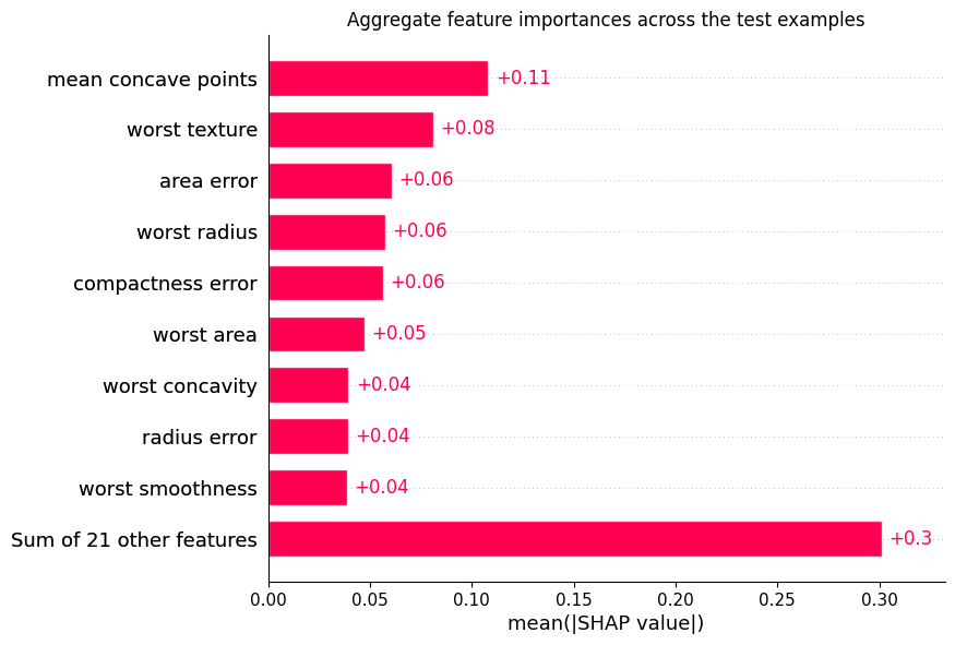
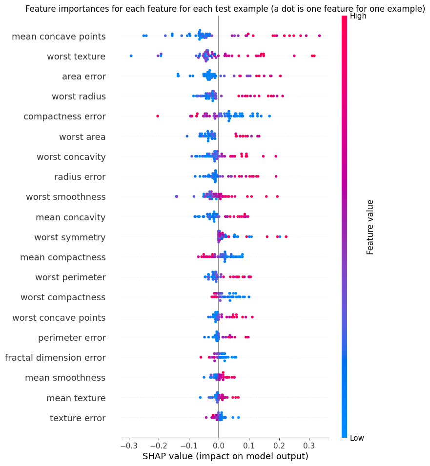
### `interpretability.shap.shapiq_to_shap_explanation`

Bridge helper that computes first-order Shapley values with a shapiq explainer
and wraps them in a `shap.Explanation` for use with `shap.plots.*` and
`shap.summary_plot`. This is the recommended way to use shap plotting with
TabPFN (see [shap\_example.py](https://github.com/PriorLabs/tabpfn-extensions/blob/main/examples/interpretability/shap_example.py)).

<Note>
  The `shap` package is **not** included in the `interpretability` extra — shapiq
  handles the computation. Install it separately to use this bridge:
  `pip install shap`
</Note>

| Parameter       | Type                | Default    | Description                                                                                    |
| --------------- | ------------------- | ---------- | ---------------------------------------------------------------------------------------------- |
| `explainer`     | `shapiq.Explainer`  | *required* | A shapiq explainer — e.g. from `get_tabpfn_imputation_explainer(..., index="SV", max_order=1)` |
| `X`             | `ndarray`           | *required* | `(n, d)` array of rows to explain                                                              |
| `budget`        | `int`               | *required* | Model evaluations per row. For exact Shapley values on `d` features, pass `2**d`.              |
| `feature_names` | `list[str] \| None` | `None`     | Feature names for `shap.plots.*` axis labels.                                                  |

**Returns:** `shap.Explanation` with `values.shape == (n, d)`. Only first-order
Shapley values are wrapped — for higher-order interactions use shapiq's native
plots directly on the `InteractionValues` object.

***

<CardGroup cols={2}>
  <Card title="FAQ" icon="question-circle" href="/faq">
    GPU setup, batch inference, and performance tuning.
  </Card>

  <Card title="Classification" icon="tags" href="/capabilities/classification">
    Binary and multi-class classification guide.
  </Card>

  <Card title="Regression" icon="chart-line" href="/capabilities/regression">
    Point estimates, quantiles, and full distributions.
  </Card>

  <Card title="Fine-Tuning" icon="sliders" href="/capabilities/fine-tuning">
    Adapt TabPFN to your domain-specific data.
  </Card>
</CardGroup>