ByPhilipp Singer
Watch a tiny TabPFN learn in-context prediction from synthetic tables alone. This cookbook is fully self-contained: it builds a small TabPFN-style tabular foundation model (nanoTabPFN), generates its synthetic pretraining data on the fly, trains it for a few minutes, and evaluates the result on real datasets it has never seen. The whole pipeline is here, in this order:
  1. The prior – a random program that produces endless synthetic classification tables.
  2. The architecture – a transformer that attends across rows and across columns of a table.
  3. In-context inference – a fit / predict_proba wrapper that does no gradient steps.
  4. Pretraining – the model learns to do Bayesian inference on tables drawn from the prior.
  5. Evaluation – zero-shot performance on iris, wine, breast cancer, and a harder dataset left as a challenge.
The model and training loop are a condensed version of nanoTabPFN (github.com/automl/nanotabpfn), a minimal re-implementation of the TabPFN v2 architecture. The surrounding tooling (prior interfaces, evaluation pipeline, pre-generated prior dumps) lives in the TFM-Playground (github.com/automl/TFM-Playground). This notebook re-implements the pieces it needs so that it runs on its own.
This is a teaching model, not the production TabPFN. To use the pretrained TabPFN on your own data, see the other cookbooks.

Setup

Everything runs on plain PyTorch. A GPU (or Apple Silicon) makes pretraining faster, but a CPU works too. In Colab, pick a GPU runtime under Runtime → Change runtime type.

The prior: where the training data comes from

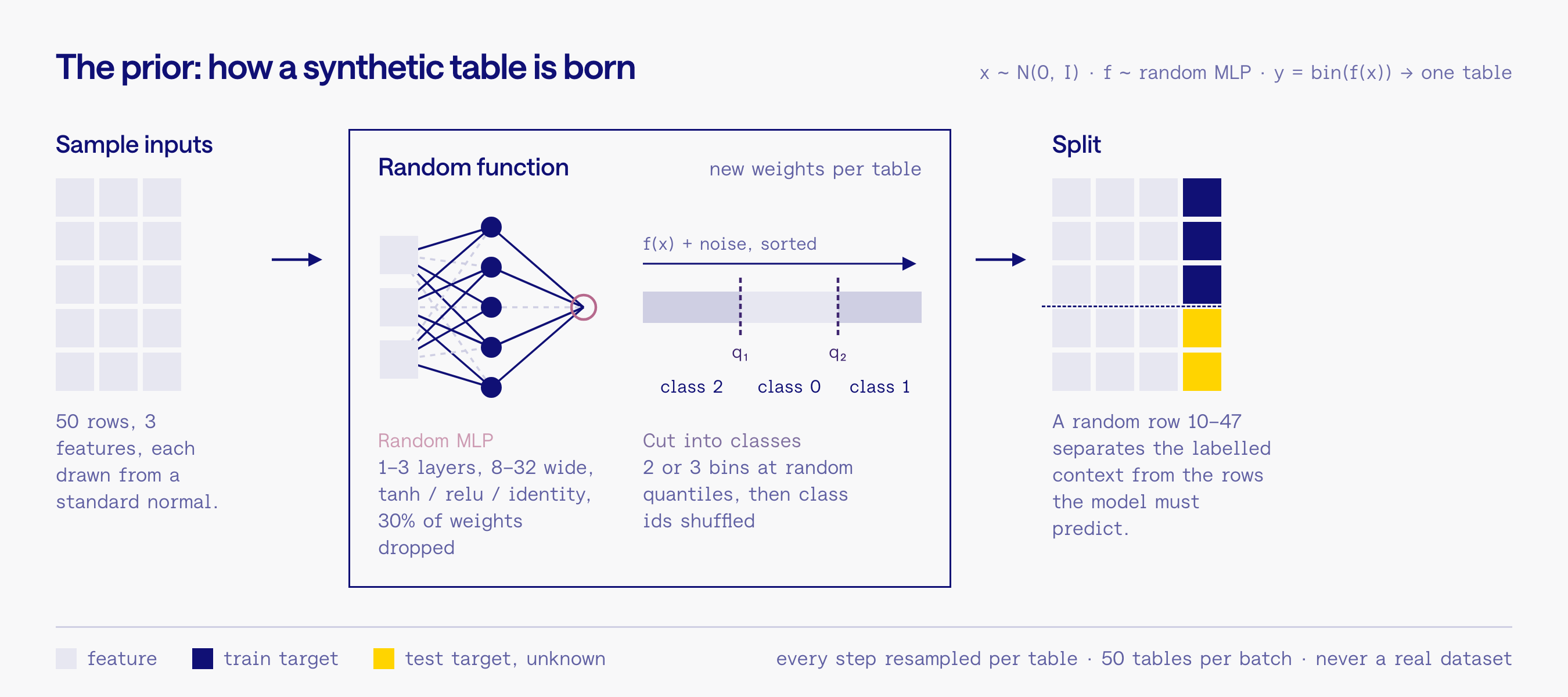
A tabular foundation model is never trained on real datasets. Instead we write down a prior over “plausible tables”: a random program that, each time it is called, invents a brand-new dataset. Here each table is produced by
  1. drawing NUM_ROWS input rows xN(0,I)x \sim \mathcal{N}(0, I) with NUM_FEATURES columns,
  2. drawing a random neural network ff (random depth, width, activation, sparse weights) and computing f(x)f(x) plus noise,
  3. cutting the scalar output at random quantiles into 2 or 3 classes, and shuffling the class ids.
Every call yields a different function, so the model can never memorize. It has to learn the algorithm: “look at the labeled rows, infer the underlying function, predict the unlabeled rows”. The generator returns exactly one dictionary per training step: x (batch, rows, features), y (batch, rows) and the index that separates the labeled “train” rows from the “test” rows the model must predict. The prior: sample inputs, random MLP, cut into classes, split
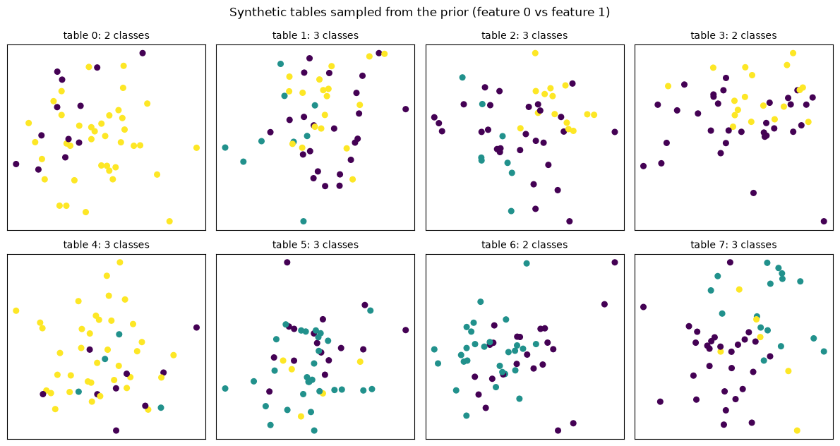
Let’s look at a few synthetic tables. Each panel is one dataset: the first two features on the axes, color is the class. Notice how different the decision regions are from table to table. That variety is what the model has to cope with.
The prior: where the training data comes from

The architecture: a transformer over table cells

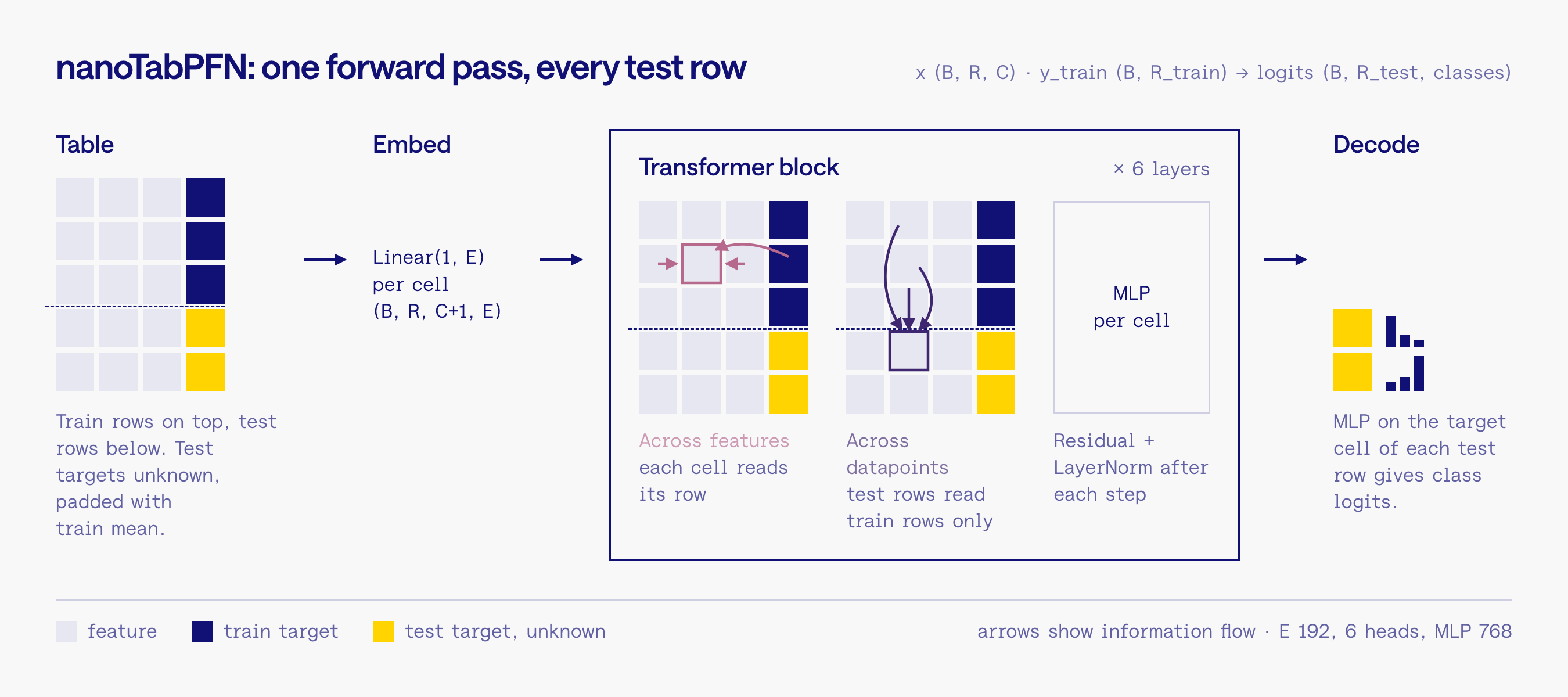
nanoTabPFN embeds every cell of the table into a vector, so a table becomes a tensor of shape (batch, rows, columns, embedding). The target column is appended as one more column; for the rows we want to predict, the target is unknown and gets padded with the mean of the known targets. Each transformer block then applies attention in two directions:
  • between features – for every row, cells attend to the other cells of the same row (which columns matter?),
  • between datapoints – for every column, rows attend to the labeled rows (which training examples are similar to me?).
Test rows only ever attend to training rows, never to each other, so predictions are independent of the other test rows. Finally a small MLP on the target-cell embedding of each test row produces the class logits. The code below follows nanoTabPFN closely, with the memory-chunking helper for large tables removed. Parameter names are identical, so checkpoints trained with the TFM-Playground scripts load into this model as well. nanoTabPFN architecture: input table, cell embeddings, two-way attention, decoder

Following the tensor shapes

The same picture in numbers. Forward hooks print the shape at every stage for one small batch. Watch how the table is flattened one way for attention between features (B*R sequences of length C+1) and the other way for attention between datapoints (B*(C+1) sequences of length R). The datapoint attention is called twice per block: once for the train rows attending to themselves and once for the test rows attending to the train rows.

In-context inference: a scikit-learn style wrapper

There is no training at fit time. fit just stores the data; predict_proba concatenates training and test rows into one table, runs a single forward pass, and applies a softmax to the logits of the test rows.

Real evaluation datasets

Four real datasets, each split 50/50. The model has never seen any of them. Note that wine has 13 features and breast cancer has 30, while the prior only ever produced 3-feature tables. Nothing in the architecture is tied to the number of columns (attention runs over however many cells a row has), so the model can still be applied. Whether it works there is an empirical question we answer below. The fourth dataset, QSAR biodegradation from OpenML, is deliberately harder: 1055 molecules described by 41 molecular descriptors, many of them skewed counts, labeled as readily biodegradable or not. We will return to it at the end.
An untrained model is at chance level or worse: a randomly initialized network is not neutral, it computes some arbitrary function of the inputs, and on breast cancer that function happens to be anti-correlated with the label. Now let’s teach it.

Pretraining

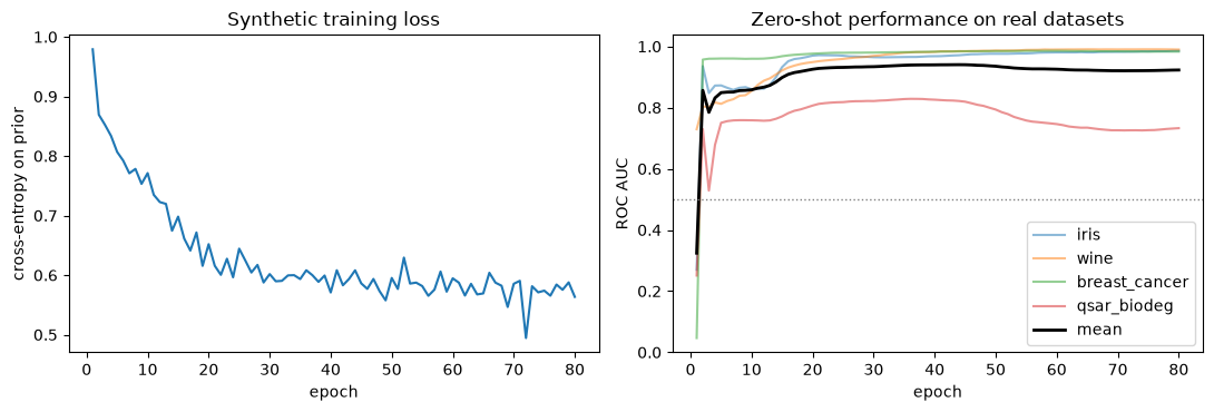
The loop is standard supervised learning with a twist: every step samples a fresh batch of tables, feeds the labeled rows plus the unlabeled features through the model, and applies cross-entropy on the test rows only. Because the model sees the labeled rows inside its input, minimizing this loss means learning to do in-context prediction. We use AdamW in its schedule-free variant so we don’t need a learning-rate schedule, plus gradient clipping. After every epoch we evaluate on the four real datasets; watch synthetic loss go down and real-data AUC go up. With the default settings (80 epochs x 25 steps x 50 tables = 100k synthetic tables) this takes about 4 minutes on an Apple M4 Max and less on a recent NVIDIA GPU. On a CPU-only runtime expect considerably longer. On the three classic datasets AUC is typically above 0.9 after 5 epochs and saturates around epoch 30, so feel free to stop early with the interrupt button; the model and the history so far are kept. Progress is printed every 5 epochs.

Training curves

Left: cross-entropy on synthetic tables. Right: ROC AUC on the four real datasets. The model has never seen a real row, yet the two curves move together.
Training curves

Before and after

Same splits, same metric, same weights up to the pretraining. fit never ran a gradient step on any of these datasets. As a reference point we add logistic regression, a classical model that is trained on each dataset.

Challenge: close the gap on QSAR biodegradation

On iris, wine and breast cancer the pretrained model matches or beats logistic regression without ever training on them. On QSAR biodegradation it does not: a plain linear model trained on the 500 labeled molecules is far ahead. Nothing about the dataset is exotic. What is off is the prior. Every synthetic table the model has ever seen had 3 Gaussian features and 50 rows; this dataset has 41 columns of skewed counts and indicator variables, several of them irrelevant, and 10 times as many rows. The model is being asked to do inference under a prior that puts almost no mass on tables like this one. The training curve says the same thing: the qsar_biodeg line rises early, peaks and then drifts down while the synthetic loss keeps improving. The longer the model specializes to the prior, the worse it fits the one dataset the prior does not describe. Your task: change the prior, the training setup or the architecture so that the pretrained model beats logistic regression on qsar_biodeg while staying strong on the other three datasets. Keep the evaluation cell as the scoreboard. The list below is a good place to start; the number of features per table and the input distribution are the most obvious mismatches.

Ideas to experiment with

Everything in this notebook is a knob. Change one thing, rerun, compare the curve and the scoreboard. If you outgrow this notebook, the TFM-Playground has the full toolkit: several pluggable priors (including the TabPFN v1 prior and pre-generated prior dumps), a regression variant, larger training runs with checkpointing and logging, and evaluation on TabArena.
  • Prior: sample the number of features per table (1 to 10) instead of fixing 3; add a second function family (random tree, Gaussian process, small causal graph) and mix them; use non-normal inputs (uniform, log-normal, categorical); add label noise, irrelevant columns, missing values, and up to 10 imbalanced classes.
  • Training: vary the row count per batch (20 to 200); more steps per epoch, fewer epochs; sweep the learning rate and try a warmup and cosine schedule; larger batches.
  • Architecture: 3 vs 12 layers; shuffle feature order during training and ensemble over permutations at inference; ablate one attention direction to see what it contributes; learned embedding for the unknown target instead of mean padding.
  • Evaluation: more datasets; log loss next to ROC AUC for calibration; accuracy vs. number of context rows.

References

  • nanoTabPFN – minimal TabPFN v2 re-implementation this notebook is based on: github.com/automl/nanotabpfn
  • TFM-Playground – open playground for tabular foundation models with prior interfaces, pre-generated prior dumps, evaluation on TabArena and a regression variant: github.com/automl/TFM-Playground