Interpretability - Prior Labs

The Interpretability Extension adds dedicated support for shapiq, along with convenience wrappers for sklearn’s built-in interpretability tools, and for plotting with the shap library (see here). Shapley values explain a single prediction by attributing the prediction’s deviation from the baseline (mean prediction) to individual features. They provide a consistent, game-theoretic measure of feature influence. Mathematically, each Shapley value represents the marginal contribution of a feature across all possible feature combinations. This can be used to:

See which features drive model predictions.
Compare feature importance across samples.
Detect feature interactions.
Debug unexpected model behavior.

Why TabPFN is Well-Suited for Interpretability

TabPFN produces smooth, well-calibrated predictions that make post-hoc explanations more stable and meaningful. Because it is a foundation model pretrained on synthetic data, it generalizes without overfitting to individual training samples — so feature attributions reflect genuine patterns. TabPFN follows the scikit-learn estimator API (fit, predict, predict_proba), which means it works out of the box with most interpretability tools in the sklearn ecosystem — partial dependence plots, permutation importance, and any other method that accepts a sklearn-compatible estimator. No wrappers or adapters needed.

Installation

pip install tabpfn "tabpfn-extensions[interpretability]"

This installs shapiq and the other dependencies needed for all methods. To run against the cloud API instead of locally, install tabpfn-client in place of tabpfn:

pip install tabpfn-client "tabpfn-extensions[interpretability]"

Quickstart

Train a model, explain a single prediction, and plot the result:

This tutorial runs TabPFN locally, which requires a GPU — see our FAQ for GPU setup. The recommended get_tabpfn_imputation_explainer relies on fit_mode="fit_with_cache", which is local-only and not available in the tabpfn_client backend. To use the cloud API, replace the tabpfn import with tabpfn_client and remove fit_mode (the client does not support it yet).

from sklearn.datasets import load_iris
from sklearn.model_selection import train_test_split
from tabpfn import TabPFNClassifier
from tabpfn_extensions.interpretability.shapiq import get_tabpfn_imputation_explainer

X, y = load_iris(return_X_y=True, as_frame=True)
X_train, X_test, y_train, y_test = train_test_split(X, y, test_size=0.2, random_state=42)

# fit_mode="fit_with_cache" engages the KV-cache fast path; set it BEFORE .fit().
clf = TabPFNClassifier(fit_mode="fit_with_cache")
clf.fit(X_train, y_train)

explainer = get_tabpfn_imputation_explainer(model=clf, data=X_train)
sv = explainer.explain(X_test.iloc[0:1].values, budget=128)
sv.plot_waterfall()

Choosing a Method

Before diving into each method, here is a summary to help you pick the right tool for the question you are trying to answer.

Two shapiq adapters — get_tabpfn_imputation_explainer uses imputation-based feature removal (marginal / conditional / baseline). The training set is fixed across coalitions, so the KV-cache fast path applies — construct the model with fit_mode="fit_with_cache". This is the recommended adapter. get_tabpfn_explainer uses the remove-and-recontextualize paradigm (Rundel et al. 2024): TabPFN is re-fit for every coalition, so the KV cache cannot be reused — expect this path to be substantially slower.

Method	What it tells you	When to reach for it	Recommended scale
shapiq (recommended)	A redesigned and improved version of the well-known SHAP library, with a more efficient and scalable implementation of Shapley values and Shapley interactions, plus native support for TabPFN. Tells you which features drove a specific prediction.	You want per-sample explanations and care about feature interactions, or you want the fastest Shapley-based method for TabPFN.	Any dataset TabPFN supports. Cost is per-sample and controlled by the `budget` parameter, so explain in batches if needed.
Partial Dependence / ICE	The global, marginal effect of one or two features across the entire dataset.	You want to understand how a feature affects the model on average rather than for a single sample, or you want to visually compare TabPFN against another sklearn estimator.	Any dataset TabPFN supports. Cost scales with grid resolution × samples, so limit to a few features at a time.
Feature Selection	Which minimal subset of features preserves model performance.	You want to simplify your model or identify redundant features before deployment.	Best under ~5,000 samples. Involves repeated cross-validation across feature subsets, so cost multiplies quickly with dataset size.

If you are still unsure which method to use, follow the table below to see the best tools for most common questions.

Question	Method
”Why did the model predict this for this sample?“	shapiq — `get_tabpfn_imputation_explainer`
”Which feature pairs interact most?“	shapiq — `get_tabpfn_imputation_explainer` with `index="k-SII"`, `max_order=2`
”How does feature X affect predictions globally?”	Partial Dependence — `partial_dependence_plots`
”How can I use the remove-and-recontextualize paradigm?“	shapiq — `get_tabpfn_explainer`
”Which features can I drop without losing accuracy?”	Feature Selection — `feature_selection`

Use Cases

Explain a prediction with shapiq

Use Shapley interaction indices to understand not just which features matter, but which feature pairs drive a prediction together.

Classification
Regression

from sklearn.datasets import load_breast_cancer
from sklearn.model_selection import train_test_split
from tabpfn import TabPFNClassifier
from tabpfn_extensions.interpretability.shapiq import get_tabpfn_imputation_explainer

X, y = load_breast_cancer(return_X_y=True, as_frame=True)
X_train, X_test, y_train, y_test = train_test_split(X, y, test_size=0.2, random_state=42)

clf = TabPFNClassifier(fit_mode="fit_with_cache")
clf.fit(X_train, y_train)

# k-SII captures pairwise feature interactions
explainer = get_tabpfn_imputation_explainer(
    model=clf,
    data=X_train,
    index="k-SII",
    max_order=2,
)

sv = explainer.explain(X_test.iloc[0:1].values, budget=128)
print(sv)              # top interactions ranked by magnitude
sv.plot_waterfall()    # waterfall plot showing additive contributions

from sklearn.datasets import load_diabetes
from sklearn.model_selection import train_test_split
from tabpfn import TabPFNRegressor
from tabpfn_extensions.interpretability.shapiq import get_tabpfn_imputation_explainer

X, y = load_diabetes(return_X_y=True, as_frame=True)
X_train, X_test, y_train, y_test = train_test_split(X, y, test_size=0.2, random_state=42)

reg = TabPFNRegressor(fit_mode="fit_with_cache")
reg.fit(X_train, y_train)

# SV with max_order=1 gives plain Shapley values (no interactions)
explainer = get_tabpfn_imputation_explainer(
    model=reg,
    data=X_train,
    index="SV",
    max_order=1,
)

sv = explainer.explain(X_test.iloc[0:1].values, budget=128)
sv.plot_waterfall()

Visualize global feature effects with Partial Dependence Plots

PDP and ICE curves show how a feature affects predictions across the whole dataset, not just one sample.

Classification
Regression

from sklearn.datasets import load_breast_cancer
from sklearn.model_selection import train_test_split
from tabpfn import TabPFNClassifier
from tabpfn_extensions.interpretability.pdp import partial_dependence_plots

X, y = load_breast_cancer(return_X_y=True, as_frame=True)
X_train, X_test, y_train, y_test = train_test_split(X, y, test_size=0.2, random_state=42)

clf = TabPFNClassifier()
clf.fit(X_train, y_train)

# PDP for two features; set kind="individual" for ICE, or "both" for overlay
partial_dependence_plots(
    clf, X_test.values,
    features=[0, 1],
    kind="average",
    target_class=1,
)

from sklearn.datasets import load_diabetes
from sklearn.model_selection import train_test_split
from tabpfn import TabPFNRegressor
from tabpfn_extensions.interpretability.pdp import partial_dependence_plots

X, y = load_diabetes(return_X_y=True, as_frame=True)
X_train, X_test, y_train, y_test = train_test_split(X, y, test_size=0.2, random_state=42)

reg = TabPFNRegressor()
reg.fit(X_train, y_train)

# 1D partial dependence for features 0 and 2, with ICE overlay
partial_dependence_plots(reg, X_test.values, features=[0, 2], kind="both")

# 2D interaction plot
partial_dependence_plots(reg, X_test.values, features=[(0, 2)])

The remove-and-recontextualize alternative

get_tabpfn_explainer uses the remove-and-recontextualize paradigm (Rundel et al. 2024): TabPFN is re-fit for every coalition, so the KV cache cannot be reused — expect this path to be substantially slower than the recommended get_tabpfn_imputation_explainer. Reach for it when you specifically want this paradigm. It also takes the training labels and does not need fit_mode.

from sklearn.datasets import load_breast_cancer
from sklearn.model_selection import train_test_split
from tabpfn import TabPFNClassifier
from tabpfn_extensions.interpretability.shapiq import get_tabpfn_explainer

X, y = load_breast_cancer(return_X_y=True, as_frame=True)
X_train, X_test, y_train, y_test = train_test_split(X, y, test_size=0.2, random_state=42)

clf = TabPFNClassifier()
clf.fit(X_train, y_train)

explainer = get_tabpfn_explainer(model=clf, data=X_train, labels=y_train)
sv = explainer.explain(X_test.iloc[0:1].values, budget=128)
sv.plot_waterfall()

Feature selection

Sequential feature selection identifies the minimal subset of features that contributes most to model performance:

from tabpfn_extensions.interpretability.feature_selection import feature_selection

result = feature_selection(clf, X_train.values, y_train.values, n_features_to_select=5)
X_selected = result.selector.transform(X_test.values)
print("Selected feature indices:", result.selected_indices)
print(f"CV score: {result.selected_score_mean:.4f} ± {result.selected_score_std:.4f}")

Controlling the budget parameter

The budget parameter in explainer.explain() sets how many coalition samples shapiq evaluates to approximate Shapley values. Each coalition is a subset of features — evaluating more of them produces more accurate estimates but costs more model calls. In theory, exact Shapley values require evaluating all 2^n feature subsets (e.g. 1024 for 10 features, ~1 billion for 30). In practice, shapiq’s approximation algorithms converge well before that:

Number of features	Suggested budget	Notes
Few features (< 10)	`64`–`128`	Converges quickly; low budgets are fine
Medium (10–20 features)	`128`–`512`	Good accuracy/speed tradeoff
Many features (20+)	`512`–`2048`	Higher budgets help, but returns diminish

Start low (e.g. budget=128) and increase only if the resulting explanations look noisy or unstable across repeated runs.

Library Reference

`interpretability.shapiq.get_tabpfn_imputation_explainer`

Creates a shapiq TabularExplainer that uses imputation-based feature removal (marginal / conditional / baseline). The training set is fixed across coalitions, so the KV-cache fast path applies — construct the model with fit_mode="fit_with_cache" (set before .fit()); the wrapper warns at construction time if it is not. This is the recommended adapter.

Parameter	Type	Default	Description
`model`	`TabPFNClassifier \| TabPFNRegressor`	required	Fitted TabPFN model
`data`	`DataFrame \| ndarray`	required	Background data for imputation sampling
`index`	`str`	`"k-SII"`	Shapley index type. Options: `"SV"` (Shapley values), `"k-SII"` (k-Shapley interaction index), `"SII"`, `"FSII"`, `"FBII"`, `"STII"`. With `max_order=1`, `"k-SII"` reduces to standard Shapley values.
`max_order`	`int`	`2`	Maximum interaction order. Set to `1` for single-feature attributions only (no interactions).
`imputer`	`str`	`"baseline"`	Imputation method. `"baseline"` uses one fixed fill value per feature (one forward pass per coalition); `"marginal"` and `"conditional"` draw multiple samples and are 50–100× slower with little gain for TabPFN.
`class_index`	`int \| None`	`None`	Class to explain for classification models. Defaults to class `1` when `None`. Ignored for regression.
`**kwargs`			Additional keyword arguments forwarded to `shapiq.TabularExplainer`

Returns: shapiq.TabularExplainer Call .explain(x, budget=N) where x is a 2D numpy array of shape (1, n_features) and budget is the number of coalition samples to evaluate (see Controlling the budget parameter). Returns a shapiq.InteractionValues object with .plot_waterfall(), .plot_force(), and other visualization methods.

`interpretability.shapiq.get_tabpfn_explainer`

Creates a shapiq TabPFNExplainer that uses the remove-and-recontextualize paradigm (Rundel et al. 2024). TabPFN is re-fit for every coalition, so the KV cache cannot be reused — expect this path to be substantially slower than the recommended get_tabpfn_imputation_explainer.

Parameter	Type	Default	Description
`model`	`TabPFNClassifier \| TabPFNRegressor`	required	Fitted TabPFN model
`data`	`DataFrame \| ndarray`	required	Background / training data
`labels`	`DataFrame \| ndarray`	required	Labels for the background data
`index`	`str`	`"k-SII"`	Shapley index type (same options as above)
`max_order`	`int`	`2`	Maximum interaction order
`class_index`	`int \| None`	`None`	Class to explain (classification only)
`**kwargs`			Additional keyword arguments forwarded to `shapiq.TabPFNExplainer`

Returns: shapiq.TabPFNExplainer Same .explain(x, budget=N) interface as above.

`interpretability.pdp.partial_dependence_plots`

Convenience wrapper around sklearn’s PartialDependenceDisplay.from_estimator.

Parameter	Type	Default	Description
`estimator`	sklearn-compatible model	required	Fitted estimator
`X`	`ndarray`	required	Input features
`features`	`list[int \| tuple[int, int]]`	required	Feature indices for 1D plots, or `(i, j)` tuples for 2D interaction plots
`grid_resolution`	`int`	`20`	Number of grid points per feature axis
`kind`	`str`	`"average"`	`"average"` for PDP, `"individual"` for ICE curves, `"both"` for overlay
`target_class`	`int \| None`	`None`	For classifiers: which class probability to plot
`ax`	`matplotlib.axes.Axes \| None`	`None`	Optional axes to plot into
`**kwargs`			Forwarded to `PartialDependenceDisplay.from_estimator`

Returns: sklearn.inspection.PartialDependenceDisplay

`interpretability.feature_selection.feature_selection`

Sequential feature selection using cross-validation. Returns a rich result object with the fitted selector, selected indices/names, and baseline vs. selected CV scores.

Parameter	Type	Default	Description
`estimator`	sklearn-compatible model	required	Fitted estimator
`X`	`ndarray`	required	Input features
`y`	`ndarray`	required	Target values
`n_features_to_select`	`int \| float \| str`	required	Number of features to keep. `int` for an absolute count, `float` for a fraction, or `"auto"` (requires `tol`).
`feature_names`	`list[str] \| None`	`None`	Feature names. When provided, `selected_names` on the result is populated.
`cv`	`int \| CV generator`	`5`	Cross-validation strategy.
`scoring`	`str \| Callable \| None`	`None`	Metric to maximize. Defaults to accuracy for classifiers, R² for regressors.
`direction`	`str`	`"forward"`	`"forward"` (add features) or `"backward"` (remove features).
`n_jobs`	`int \| None`	`None`	Parallelism over candidate features per round. `-1` for all cores.
`tol`	`float \| None`	`None`	Stop threshold for `n_features_to_select="auto"`.
`verbose`	`bool`	`True`	Print per-round progress and CV scores.
`**kwargs`			Forwarded to `sklearn.feature_selection.SequentialFeatureSelector`.

Returns: FeatureSelectionResult — a dataclass with the following attributes:

Attribute	Type	Description
`selector`	`SequentialFeatureSelector`	Fitted selector. Call `.transform(X)` to project to selected columns.
`support_mask`	`ndarray`	Boolean mask of shape `(n_features,)`.
`selected_indices`	`list[int]`	Integer indices of selected features.
`selected_names`	`list[str] \| None`	Selected feature names; `None` if `feature_names` was not passed.
`baseline_score_mean`	`float`	Mean CV score on all features before selection.
`baseline_score_std`	`float`	Std of the baseline CV score.
`selected_score_mean`	`float`	Mean CV score on the selected feature subset.
`selected_score_std`	`float`	Std of the selected-subset CV score.

`interpretability.shap.shapiq_to_shap_explanation`

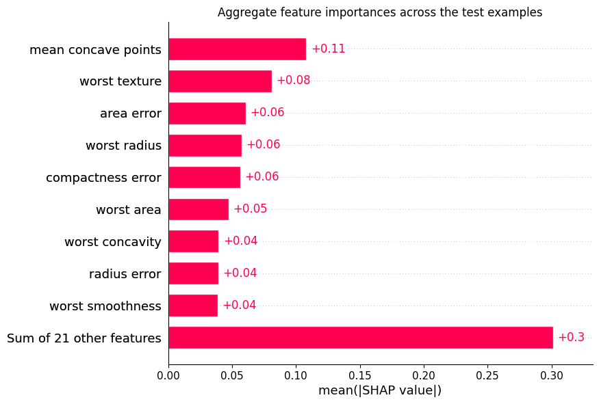
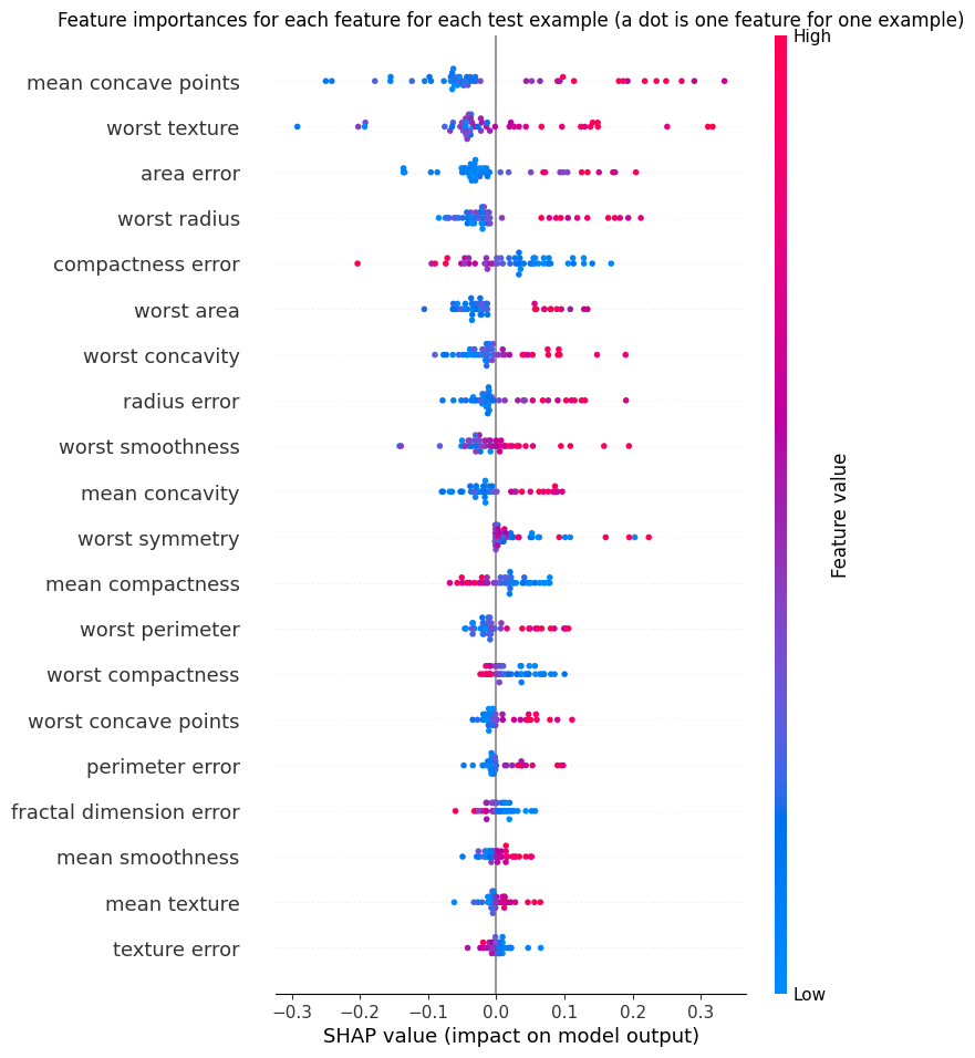
Bridge helper that computes first-order Shapley values with a shapiq explainer and wraps them in a shap.Explanation for use with shap.plots.* and shap.summary_plot. This is the recommended way to use shap plotting with TabPFN (see shap_example.py).

The shap package is not included in the interpretability extra — shapiq handles the computation. Install it separately to use this bridge: pip install shap

Parameter	Type	Default	Description
`explainer`	`shapiq.Explainer`	required	A shapiq explainer — e.g. from `get_tabpfn_imputation_explainer(..., index="SV", max_order=1)`
`X`	`ndarray`	required	`(n, d)` array of rows to explain
`budget`	`int`	required	Model evaluations per row. For exact Shapley values on `d` features, pass `2**d`.
`feature_names`	`list[str] \| None`	`None`	Feature names for `shap.plots.*` axis labels.

Returns: shap.Explanation with values.shape == (n, d). Only first-order Shapley values are wrapped — for higher-order interactions use shapiq’s native plots directly on the InteractionValues object.

FAQ

GPU setup, batch inference, and performance tuning.

Classification

Binary and multi-class classification guide.

Regression

Point estimates, quantiles, and full distributions.

Fine-Tuning

Adapt TabPFN to your domain-specific data.

​Why TabPFN is Well-Suited for Interpretability

​Installation

​Quickstart

​Choosing a Method

​Use Cases

​Explain a prediction with shapiq

​Visualize global feature effects with Partial Dependence Plots

​The remove-and-recontextualize alternative

​Feature selection

​Controlling the budget parameter

​Library Reference

​interpretability.shapiq.get_tabpfn_imputation_explainer

​interpretability.shapiq.get_tabpfn_explainer

​interpretability.pdp.partial_dependence_plots

​interpretability.feature_selection.feature_selection

​interpretability.shap.shapiq_to_shap_explanation

FAQ

Classification

Regression

Fine-Tuning

Why TabPFN is Well-Suited for Interpretability

Installation

Quickstart

Choosing a Method

Use Cases

Explain a prediction with shapiq

Visualize global feature effects with Partial Dependence Plots

The remove-and-recontextualize alternative

Feature selection

Controlling the budget parameter

Library Reference

`interpretability.shapiq.get_tabpfn_imputation_explainer`

`interpretability.shapiq.get_tabpfn_explainer`

`interpretability.pdp.partial_dependence_plots`

`interpretability.feature_selection.feature_selection`

`interpretability.shap.shapiq_to_shap_explanation`