Bayesian Optimization with TabPFN Extensions

ByKlemens FlögeTuana Çelik

Use TabPFN as the surrogate model inside a Bayesian optimization loop. This cookbook turns the tabpfn-extensions Bayesian optimization example into a step-by-step notebook. We optimize the 4D Rosenbrock benchmark, compare TabPFN-driven search against random search under the same evaluation budget, and show how propose_next_point() uses the predictive distribution from TabPFN to compute Expected Improvement (EI). 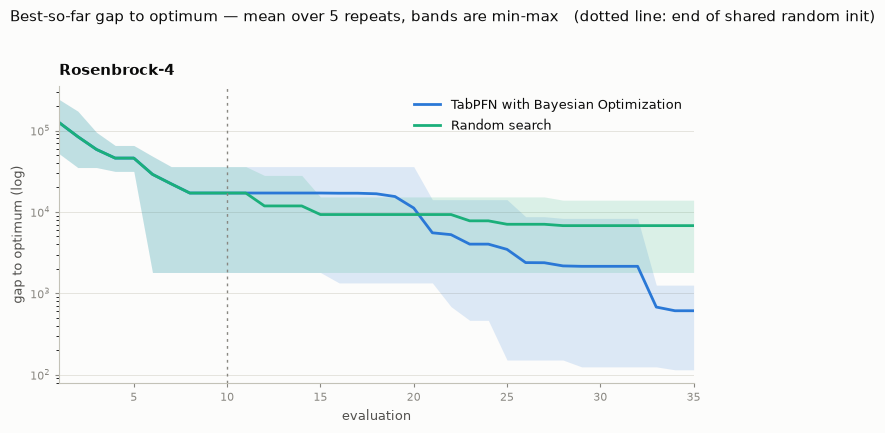A single run tells you very little — the starting design alone can decide the outcome. So we repeat the whole experiment 5 times with different random inits and report the mean with a min–max band. Relevant resources:

Setup

Install the full TabPFN package plus the Bayesian optimization extras from tabpfn-extensions. This example uses the local PyTorch-backed TabPFN implementation because the optimizer refines candidates with gradients (differentiable_input=True).

%pip install -q -U "tabpfn-extensions[bayesian-optimization]" "tabpfn>=8.1.0" "tqdm>=4.63.0,<=4.67.3" matplotlib

TabPFN as the surrogate, BoTorch for the benchmark objective, and Matplotlib for a quick comparison plot.

import matplotlib.pyplot as plt
import numpy as np
import torch
from botorch.test_functions import Rosenbrock
from tqdm.auto import trange

from tabpfn import TabPFNRegressor
from tabpfn_extensions.bayesian_optimization import propose_next_point

The Optimization Problem

Rosenbrock-4 is a four-dimensional benchmark with a narrow, curved valley: easy to fall into, hard to walk along. Its optimum is 0.0 at (1, 1, 1, 1), and random search burns most of its budget far outside the valley. The TabPFN surrogate predicts a full bar distribution over the objective value. propose_next_point() uses that predictive distribution to compute Expected Improvement, then refines the most promising candidates with gradient ascent on the acquisition function itself. Two details worth calling out:

negate=True turns the minimization benchmark into a maximization problem, which is what EI expects; optimal_value follows the sign.
The optimizer searches the unit cube [0, 1]^4, but Rosenbrock lives on [-5, 10]^4, so every candidate is mapped onto the problem’s own bounds before evaluation.

N_INIT = 10
N_BO_STEPS = 25
N_SEEDS = 5
N_CANDIDATES = 512
TOP_K = 4
N_REFINE_STEPS = 8
REFINE_LR = 0.05
GAP_FLOOR = 1e-3  # the log axis needs a positive floor

DEVICE = "cuda" if torch.cuda.is_available() else "cpu"
print(f"Device: {DEVICE}")

# EI maximizes the objective, so we negate Rosenbrock to turn its optimum into a maximum.
objective = Rosenbrock(dim=4, negate=True).to(DEVICE)
LO, HI = objective.bounds[0], objective.bounds[1]
# `optimal_value` comes back as -0.0 after negation; `+ 0.0` normalises the sign.
print(f"Objective optimum: {objective.optimal_value + 0.0:.4f} on {LO.tolist()}..{HI.tolist()}")


def evaluate(unit_x: torch.Tensor) -> torch.Tensor:
    """Evaluate the benchmark on points given in the unit cube."""
    return objective(LO + unit_x * (HI - LO))

Device: cpu
Objective optimum: 0.0000 on [-5.0, -5.0, -5.0, -5.0]..[10.0, 10.0, 10.0, 10.0]

Build the TabPFN Surrogate

The critical switch is differentiable_input=True. That flag keeps gradients flowing from the acquisition value back into the candidate coordinates during refinement. We use a single estimator to stay close to the upstream example and keep runtime short on CPU. Each repeat gets its own surrogate, seeded with that repeat’s index, so the runs are independent.

def make_surrogate(seed: int) -> TabPFNRegressor:
    return TabPFNRegressor(
        n_estimators=1,
        device=DEVICE,
        random_state=seed,
        inference_precision=torch.float32,
        differentiable_input=True,
    )

Run Bayesian Optimization

Seed with random points, then let TabPFN propose the next evaluation point. Each iteration fits TabPFN on all observed evaluations so far, screens a random candidate pool with Expected Improvement, and refines the top candidates by gradient ascent before returning the next point to evaluate. We run that loop N_SEEDS = 5 times. Within a repeat, both methods start from the same N_INIT random evaluations, so the two curves can only diverge once the acquisition function takes over.

def run_bo(init_x: torch.Tensor, init_y: torch.Tensor, seed: int) -> torch.Tensor:
    """Run the loop from a fixed random init and return every observed y."""
    reg = make_surrogate(seed)
    train_x, train_y = init_x.clone(), init_y.clone()
    for _ in trange(N_BO_STEPS, desc=f"repeat {seed}", leave=False):
        next_x = propose_next_point(
            reg,
            train_x,
            train_y,
            n_candidates=N_CANDIDATES,
            top_k=TOP_K,
            n_refine_steps=N_REFINE_STEPS,
            refine_lr=REFINE_LR,
        )
        train_x = torch.cat([train_x, next_x.unsqueeze(0)])
        train_y = torch.cat([train_y, evaluate(next_x.unsqueeze(0))])
    return train_y


def gap_to_optimum(y: torch.Tensor) -> np.ndarray:
    """Best-so-far distance to the known optimum — lower is better."""
    best = np.maximum.accumulate(y.detach().cpu().numpy())
    return np.maximum(objective.optimal_value - best, GAP_FLOOR)


bo_gaps, random_gaps = [], []

for seed in range(N_SEEDS):
    # One shared init per repeat: both methods see the same starting evaluations.
    torch.manual_seed(seed)
    init_x = torch.rand(N_INIT, objective.dim, device=DEVICE)
    init_y = evaluate(init_x)

    torch.manual_seed(1000 + seed)
    bo_y = run_bo(init_x, init_y, seed)

    torch.manual_seed(1000 + seed)
    random_y = torch.cat([init_y, evaluate(torch.rand(N_BO_STEPS, objective.dim, device=DEVICE))])

    bo_gaps.append(gap_to_optimum(bo_y))
    random_gaps.append(gap_to_optimum(random_y))
    print(
        f"repeat {seed}: TabPFN gap {bo_gaps[-1][-1]:9.4g} | "
        f"random search gap {random_gaps[-1][-1]:9.4g}"
    )

bo_gap = np.array(bo_gaps)          # (N_SEEDS, N_INIT + N_BO_STEPS)
random_gap = np.array(random_gaps)

repeat 0: TabPFN gap       115 | random search gap      9698
repeat 1: TabPFN gap     124.9 | random search gap      1806
repeat 2: TabPFN gap       990 | random search gap      2376
repeat 3: TabPFN gap      1262 | random search gap      6125
repeat 4: TabPFN gap     564.6 | random search gap 1.397e+04

Compare Against Random Search

Same objective, same budget, same starting points — only the choice of the next point differs. Rosenbrock values span several orders of magnitude, so we report the gap to the optimum (optimum - best so far) rather than the raw objective. Lower is better.

for name, gaps in [("TabPFN", bo_gap), ("Random search", random_gap)]:
    final = gaps[:, -1]
    print(
        f"{name:<14} final gap over {N_SEEDS} repeats: "
        f"mean {final.mean():9.4g} | median {np.median(final):9.4g} | best {final.min():9.4g}"
    )

TabPFN         final gap over 5 repeats: mean     611.2 | median     564.6 | best       115
Random search  final gap over 5 repeats: mean      6795 | median      6125 | best      1806

evals = np.arange(1, bo_gap.shape[1] + 1)

fig, ax = plt.subplots(figsize=(7.2, 4.2), facecolor="#fcfcfb")
ax.set_facecolor("#fcfcfb")
ax.set_yscale("log")

# Mean over repeats, band spans min-max across them.
for curves, label, color in [
    (bo_gap, "TabPFN with Bayesian Optimization", "#2a78d6"),
    (random_gap, "Random search", "#1baf7a"),
]:
    ax.fill_between(evals, curves.min(0), curves.max(0), color=color, alpha=0.15, lw=0)
    ax.plot(evals, curves.mean(0), color=color, lw=2, label=label)
ax.axvline(N_INIT, color="#898781", lw=1, ls=(0, (2, 3)))

ax.set_title("Rosenbrock-4", fontsize=11, color="#0b0b0b", loc="left", fontweight="bold", pad=8)
ax.grid(visible=True, axis="y", color="#e1e0d9", linewidth=0.6)
ax.set_axisbelow(True)
for side in ("top", "right"):
    ax.spines[side].set_visible(False)
for side in ("left", "bottom"):
    ax.spines[side].set_color("#c3c2b7")
ax.tick_params(colors="#898781", labelsize=8, length=3)
ax.set_xlim(1, N_INIT + N_BO_STEPS)
ax.set_xlabel("evaluation", fontsize=9, color="#52514e")
ax.set_ylabel("gap to optimum (log)", fontsize=9, color="#52514e")
ax.legend(frameon=False, fontsize=9.5, labelcolor="#0b0b0b")

fig.suptitle(
    f"Best-so-far gap to optimum — mean over {N_SEEDS} repeats, bands are min-max"
    "   (dotted line: end of shared random init)",
    fontsize=11,
    color="#0b0b0b",
    x=0.02,
    ha="left",
    y=1.02,
)
fig.tight_layout()
plt.show()

Takeaways

tabpfn-extensions already provides the Bayesian Optimization loop primitive: propose_next_point()
On Rosenbrock-4, TabPFN with Bayesian Optimization should close the gap to the optimum faster than random search under the same evaluation budget.
For more background, start with the upstream example and the tabpfn-extensions repo.

​Setup

​The Optimization Problem

​Build the TabPFN Surrogate

​Run Bayesian Optimization

​Compare Against Random Search

​Takeaways