Insurance Claim Modeling: TabPFN vs. GLM

ByPhilipp Singer

Better risk ranking and per-policy uncertainty from the raw dataframe, no feature engineering. Insurance claim data is zero-inflated: most policies never claim, and the few that do produce heavily right-skewed amounts. Pricing it well is the core actuarial problem, and the classic recipe is a two-stage generalized linear model (GLM): a frequency model (how often do claims happen?) times a severity model (how large are they?). Making a GLM work takes real feature engineering, binning, one-hot encoding, log-scaling, and choosing link functions and a Tweedie power by hand. TabPFN is a tabular foundation model that learns in a single forward pass with no per-dataset training and no preprocessing, you hand it the raw dataframe (mixed numeric and string columns, missing values and all). This notebook puts TabPFN head-to-head with matching scikit-learn GLM baselines on the standard French Motor Third-Party Liability (freMTPL2) dataset. For both the GLM and TabPFN we run the two classic recipes, a single-stage direct model and the two-stage frequency × severity (occurrence × severity) decomposition, so every comparison is like-for-like. Bottom line up front:

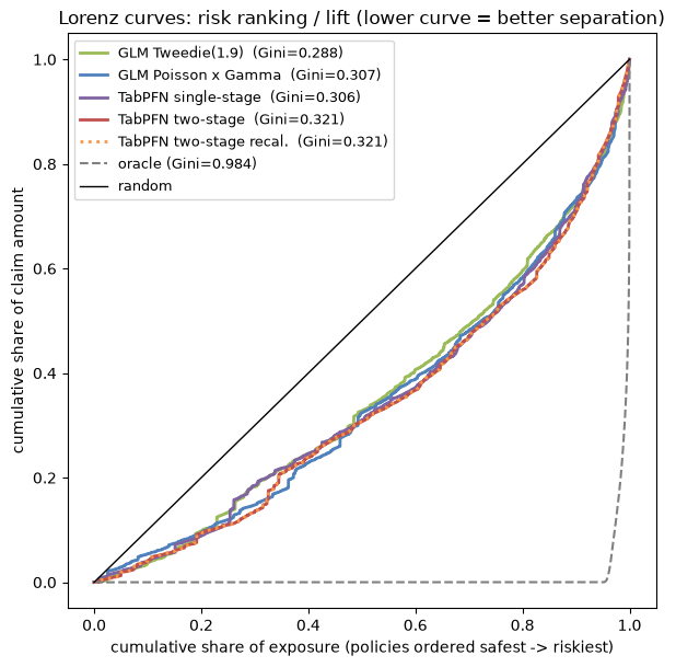
Better risk ranking, zero feature engineering. Straight from the 9-column raw dataframe, TabPFN reaches an exposure-weighted Gini of ~0.32 vs ~0.31 for the best hand-built GLM, better separation of safe from risky policies, which is what drives pricing.
Per-policy uncertainty for free. TabPFN returns a full predictive distribution per policy, so you can read the expected claim and the tail (“how bad could this one get?”), the GLM gives you only a fitted mean.
Calibration on par, with one optional line. With a single portfolio-level rescale — the same balancing a log-link GLM does implicitly — TabPFN matches the GLM on calibration while leaving the ranking untouched.

We score with the metrics actuaries actually use: the exposure-weighted Gini (ranking / lift) and Tweedie deviance / D² (calibration, the standard loss for zero-inflated cost; both are defined in the Metrics section below).

Requirements. This notebook runs on the hosted TabPFN client (tabpfn-client), so no local GPU is needed; you just need a free API token (see the setup cells below). Baselines, dataset explanation and metrics follow scikit-learn’s Tweedie regression on insurance claims example which motivated this tutorial.

!pip install tabpfn_client matplotlib scikit-learn

import warnings

import numpy as np
import pandas as pd
import matplotlib.pyplot as plt

from sklearn.datasets import fetch_openml
from sklearn.model_selection import train_test_split
from sklearn.compose import ColumnTransformer
from sklearn.pipeline import Pipeline, make_pipeline
from sklearn.preprocessing import (
    KBinsDiscretizer, OneHotEncoder, StandardScaler, FunctionTransformer,
)
from sklearn.linear_model import PoissonRegressor, GammaRegressor, TweedieRegressor
from sklearn.metrics import mean_tweedie_deviance, d2_tweedie_score, auc


# Benign numeric overflow in TabPFN's inverse target transform (expm1 on the far
# tail of the output distribution's support); results are unaffected.
warnings.filterwarnings("ignore", message="overflow encountered in exp")

RANDOM_STATE = 0
N_ESTIMATORS = 8
FEATURES = ["VehAge", "DrivAge", "VehBrand", "VehPower", "VehGas",
            "Region", "Area", "BonusMalus", "Density"]

In this notebook, we use the TabPFN client to access the API, so no hardware is required to run the model.

from tabpfn_client import TabPFNClassifier, TabPFNRegressor, get_access_token
token = get_access_token()

# uncomment for local version
# from tabpfn import TabPFNClassifier, TabPFNRegressor

The data

Each row is an insurance policy — a contract between the insurer and a policyholder — described by driver age, vehicle age, vehicle power, region, and so on. A claim is a request for compensation; the claim amount is what the insurer pays out. Exposure is how long the policy was actually observed, measured in years: a policy on the books for the full period has Exposure = 1.0, one observed for six months has Exposure ≈ 0.5. It matters because a policy watched for two months has had far less opportunity to claim than one watched all year, so every rate below is expressed per unit of exposure. Our target is the pure premium: the expected claim cost per unit of exposure, i.e., the break-even price of the risk. There are two classic ways to model it:

Single-stage: model the total claim cost per unit exposure directly.
Two-stage: model the claim frequency (claims per year) and the severity (average amount per claim) separately, then multiply.

The column reMTPL2freq holds one row per policy (risk features, claim count ClaimNb, and Exposure), freMTPL2sev holds the individual claim amounts. We aggregate claim amounts per policy and join; policies with no claim get ClaimAmount = 0. We apply the same light cleaning as the scikit-learn example (cap extreme values, make ClaimNb consistent with ClaimAmount) and derive the targets Frequency = ClaimNb / Exposure, AvgClaimAmount = ClaimAmount / ClaimNb, and PurePremium = ClaimAmount / Exposure. Note the feature columns: VehBrand, VehGas, Region, Area are strings, the rest are numeric on very different scales. A GLM cannot consume this directly; TabPFN can.

freq = fetch_openml(data_id=41214, as_frame=True).frame   # policies: features + ClaimNb + Exposure
sev = fetch_openml(data_id=41215, as_frame=True).frame     # individual claim amounts

df = freq.copy()
df["ClaimAmount"] = df["IDpol"].map(sev.groupby("IDpol")["ClaimAmount"].sum()).fillna(0.0)

# Standard cleaning.
df["ClaimNb"] = df["ClaimNb"].clip(upper=4)
df["Exposure"] = df["Exposure"].clip(upper=1)
df["ClaimAmount"] = df["ClaimAmount"].clip(upper=200_000)
df.loc[(df["ClaimAmount"] == 0) & (df["ClaimNb"] >= 1), "ClaimNb"] = 0

# Insurance companies are interested in modeling the Pure Premium, that is
# the expected total claim amount per unit of exposure for each policyholder
# in their portfolio:
df["PurePremium"] = df["ClaimAmount"] / df["Exposure"]

# This can be indirectly approximated by a 2-step modeling: the product of the
# Frequency times the average claim amount per claim:
df["Frequency"] = df["ClaimNb"] / df["Exposure"]
df["AvgClaimAmount"] = df["ClaimAmount"] / np.fmax(df["ClaimNb"], 1)

zero = (df["ClaimAmount"] == 0).mean()
print(f"{len(df):,} policies | {100 * zero:.1f}% have ZERO claim amount | "
      f"{(df.ClaimAmount > 0).sum():,} claims")
df[FEATURES + ["Exposure", "ClaimNb", "ClaimAmount", "PurePremium", "Frequency", "AvgClaimAmount"]].sort_values("ClaimAmount", ascending=False).head()

678,013 policies | 96.3% have ZERO claim amount | 24,944 claims
        VehAge  DrivAge VehBrand  VehPower     VehGas Region Area  BonusMalus  \
147894       1       21       B3         7   'Diesel'    R53    C          90
396360      18       78      B10         7  'Regular'    R93    E          50
231941      13       21       B1         4   'Diesel'    R24    A         140
270621      14       18       B2         4  'Regular'    R82    D         100
609318       2       33      B12        10  'Regular'    R94    D          80

        Density  Exposure  ClaimNb  ClaimAmount   PurePremium  Frequency  \
147894      108      0.85        1     200000.0  2.352941e+05   1.176471
396360     4762      0.58        1     200000.0  3.448276e+05   1.724138
231941       37      0.16        2     200000.0  1.250000e+06  12.500000
270621      863      0.32        1     200000.0  6.250000e+05   3.125000
609318      645      0.53        2     200000.0  3.773585e+05   3.773585

        AvgClaimAmount
147894        200000.0
396360        200000.0
231941        100000.0
270621        200000.0
609318        100000.0

fig, ax = plt.subplots(1, 2, figsize=(11, 3.6))
ax[0].bar(["no claim", "claim"],
          [(df.ClaimAmount == 0).mean(), (df.ClaimAmount > 0).mean()],
          color=["#9aa7b0", "#c0504d"])
ax[0].set_ylabel("fraction of policies")
ax[0].set_title("Zero-inflation: ~96% of policies never claim")

pos = df.loc[df.ClaimAmount > 0, "ClaimAmount"]
ax[1].hist(np.log10(pos), bins=50, color="#c0504d")
ax[1].set_xlabel("log10(ClaimAmount)")
ax[1].set_title("Severity is heavy-tailed | given a claim")
plt.tight_layout()
plt.show()

We hold out 25% of policies for testing with a random split. A production pricing model would usually be validated out of time (train on older policy years, test on newer) to catch drift, but freMTPL2 ships without a usable time index, so we follow the scikit-learn example and split at random; a simplification worth remembering for similar use cases.

df_train, df_test = train_test_split(df, test_size=0.25, random_state=RANDOM_STATE)
pp_true = df_test["PurePremium"].to_numpy()
weight = df_test["Exposure"].to_numpy()          # exposure-weighting for the metrics
print(f"train {len(df_train):,} | test {len(df_test):,}")

train 508,509 | test 169,504

Metrics

Two questions matter for a pricing model, and they need different metrics. Ranking / lift — does the model sort safe from risky policies? This is what segmentation and pricing rely on, and our headline metric. We use the exposure-weighted Gini. Sort policies from safest to riskiest by predicted premium, then trace the cumulative share of actual claim cost against the cumulative share of exposure — the Lorenz curve

L(u)

. The Gini is (twice) the area between that curve and the diagonal:

\mathrm{Gini} = 1 - 2\int_0^1 L(u)\,du

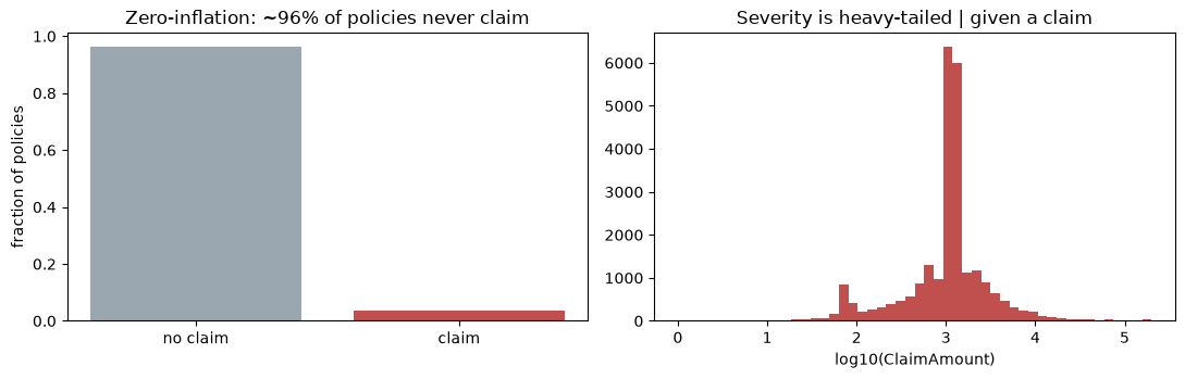
Higher is better; a model with no information scores 0. In code it is 1 - 2 * auc(cum_exposure, cum_claims). Calibration — is the predicted premium level right? We use the Tweedie deviance (lower is better) and its normalized cousin D² (higher is better, an R²-style score), the standard loss for zero-inflated, right-skewed cost targets. This is exactly the GLM’s own training objective. We deliberately skip MAE (degenerate on a 96%-zero target — it rewards predicting near-zero for everyone) and RMSE (dominated by a handful of catastrophic claims).

def gini_exposure(y_true, y_pred, exposure):
    order = np.argsort(y_pred)                     # ascending: safest -> riskiest
    exp = np.asarray(exposure)[order]
    claim = np.asarray(y_true)[order] * exp
    cum_claim = np.cumsum(claim) / claim.sum()
    cum_exp = np.cumsum(exp) / exp.sum()
    return 1 - 2 * auc(cum_exp, cum_claim)

def scores(pred):
    pred = np.clip(pred, 1e-6, None)               # Tweedie deviance needs strictly positive
    return {
        "Gini (exposure)  up": gini_exposure(pp_true, pred, weight),
        "D2 (Tweedie 1.9)  up": d2_tweedie_score(pp_true, pred, sample_weight=weight, power=1.9),
        "Tweedie dev 1.9  down": mean_tweedie_deviance(pp_true, pred, sample_weight=weight, power=1.9),
        "Tweedie dev 1.5  down": mean_tweedie_deviance(pp_true, pred, sample_weight=weight, power=1.5),
    }

GLM baselines

A GLM (generalized linear model) is a linear model with a link function — here a log link, so predictions stay positive. Being linear, every feature has to be hand-engineered into a numeric design matrix: bin the skewed numerics, one-hot the categoricals, log-and-scale the heavy-tailed one. On that shared design matrix we fit the two classic recipes for the pure premium — a single-stage direct Tweedie model, then the two-stage frequency × severity product. The hyperparameters (Tweedie power, regularization strengths) are taken straight from the scikit-learn tutorial and left untuned; in practice you would grid-search them. That cuts both ways in this comparison — TabPFN is also run untuned, on its defaults.

Single-stage GLM: direct Tweedie on pure premium

The simplest recipe: one TweedieRegressor fit straight on PurePremium, weighted by Exposure. No occurrence/severity split — a single model for the whole target. We set power=1.9 following the scikit-learn tutorial.

def make_glm_preprocessor():
    # A fresh ColumnTransformer per model (so fitting one does not overwrite another).
    log_scale = make_pipeline(FunctionTransformer(np.log, validate=False), StandardScaler())
    return ColumnTransformer([
        ("binned", KBinsDiscretizer(n_bins=10, random_state=RANDOM_STATE), ["VehAge", "DrivAge"]),
        ("onehot", OneHotEncoder(handle_unknown="ignore"),
         ["VehBrand", "VehPower", "VehGas", "Region", "Area"]),
        ("passthrough", "passthrough", ["BonusMalus"]),
        ("log_scaled", log_scale, ["Density"]),
    ], remainder="drop")

Xtr = df_train[FEATURES]
n_design = make_glm_preprocessor().fit_transform(Xtr).shape[1]
print(f"GLM design matrix: {n_design} engineered columns from {len(FEATURES)} raw features")

# Single-stage: a direct Tweedie model on the pure premium, weighted by exposure.
glm_tweedie = Pipeline([("prep", make_glm_preprocessor()),
                        ("reg", TweedieRegressor(power=1.9, alpha=0.1, max_iter=1000))])
glm_tweedie.fit(Xtr, df_train["PurePremium"], reg__sample_weight=df_train["Exposure"])
pp_glm_tweedie = glm_tweedie.predict(df_test[FEATURES])
scores(pp_glm_tweedie)

GLM design matrix: 75 engineered columns from 9 raw features
{'Gini (exposure)  up': 0.28834550102009937,
 'D2 (Tweedie 1.9)  up': 0.013735296391564011,
 'Tweedie dev 1.9  down': 33.878261888130645,
 'Tweedie dev 1.5  down': 76.40873870601743}

Two-stage GLM: frequency × severity

The classic actuarial product: a Poisson frequency model (how often claims happen, weighted by exposure) times a Gamma severity model (average amount per claim, fit on claim rows only and weighted by claim count). Their product is the expected cost per unit exposure. Again, we follow the scikit-learn tutorial and set the hyperparameters accordingly.

# Stage 1 - frequency: Poisson, weighted by exposure.
glm_freq = Pipeline([("prep", make_glm_preprocessor()),
                     ("reg", PoissonRegressor(alpha=1e-4, max_iter=500))])
glm_freq.fit(Xtr, df_train["Frequency"], reg__sample_weight=df_train["Exposure"])

# Stage 2 - severity: Gamma on claim rows only, weighted by claim count.
claim = df_train["ClaimAmount"] > 0
glm_sev = Pipeline([("prep", make_glm_preprocessor()),
                    ("reg", GammaRegressor(alpha=10.0, max_iter=500))])
glm_sev.fit(Xtr[claim.values], df_train.loc[claim, "AvgClaimAmount"],
            reg__sample_weight=df_train.loc[claim, "ClaimNb"])

pp_glm_product = glm_freq.predict(df_test[FEATURES]) * glm_sev.predict(df_test[FEATURES])
scores(pp_glm_product)

{'Gini (exposure)  up': 0.30667623396467025,
 'D2 (Tweedie 1.9)  up': 0.014606241449514612,
 'Tweedie dev 1.9  down': 33.84834486417605,
 'Tweedie dev 1.5  down': 76.15988353558402}

TabPFN

Now the same problem with TabPFN — but we feed the raw dataframe: strings, integers and floats together, no encoding, no scaling, no binning, no per-dataset tuning. GLMs fold exposure in through sample_weight and an offset. TabPFN has neither, so we hand it the information directly instead:

Exposure becomes an ordinary input feature. TabPFN learns its effect from the data rather than you specifying it as an offset. We model the bounded ClaimAmount rather than the exploding per-exposure PurePremium (dividing a claim by a tiny exposure blows up the tail).
The pure premium is read off with a counterfactual query. We predict every test policy at a full year of exposure (Exposure = 1.0), so the output is already the expected cost per unit of exposure, no division needed.

Single-stage TabPFN: regress the claim amount directly

Start with the simplest thing that could work: hand a single TabPFNRegressor the raw, 96%-zero ClaimAmount and query at full exposure. One .fit(), one .predict(), default settings — nothing else. .predict() returns the mean of TabPFN’s predicted distribution, the estimator of expected cost.

tab_features = FEATURES + ["Exposure"]
X_tr = df_train[tab_features]

# Counterfactual test set: every policy evaluated at a FULL year of exposure.
X_te_unit = df_test[tab_features].copy()
X_te_unit["Exposure"] = 1.0

reg_single = TabPFNRegressor(n_estimators=N_ESTIMATORS, ignore_pretraining_limits=True)
reg_single.fit(X_tr, df_train["ClaimAmount"])
pp_single_vanilla = reg_single.predict(X_te_unit)   # plain mean point-estimate
scores(pp_single_vanilla)

The ranking is already competitive, the Gini lands in the same range as the two stage GLM, but the calibration is off: the Tweedie deviance is enormous and D² is deeply negative. TabPFN’s default target handling is not built for a target that is 96% zeros with a heavy tail on the rest. The fix is the same one the GLMs bake in through their log link: model the target on a log scale. TabPFN exposes this as a target transform, 1_plus_log (fit on log(1 + y), invert on output), the natural choice for monetary amounts. This is the one modeling knob we touch.

reg_single = TabPFNRegressor(
    n_estimators=N_ESTIMATORS, ignore_pretraining_limits=True,
    inference_config={"REGRESSION_Y_PREPROCESS_TRANSFORMS": ("1_plus_log",)},
)
reg_single.fit(X_tr, df_train["ClaimAmount"])
pp_tabpfn_single = reg_single.predict(X_te_unit)    # plain mean point-estimate
scores(pp_tabpfn_single)

{'Gini (exposure)  up': 0.3062529264409002,
 'D2 (Tweedie 1.9)  up': -0.1560920028968369,
 'Tweedie dev 1.9  down': 39.71184155492424,
 'Tweedie dev 1.5  down': 98.82921431822498}

Results show that the ranking quality stays intact, while we severely improve the calibration quality.

Two-stage TabPFN: occurrence × severity

The actuarial decomposition, with no Poisson/Gamma machinery, just two TabPFN models:

Stage 1 — occurrence: a TabPFNClassifier for P(claim > 0).
Stage 2 — severity: a TabPFNRegressor for E[ClaimAmount | claim > 0], trained on claim rows only.

Expected cost is P(claim) × severity. Both stages are queried at Exposure = 1.0, so the product is already the pure premium. We use each stage’s mean here; the next section pulls stage 2’s full predictive distribution for a handful of example policies.

# Stage 1: occurrence  P(claim > 0 | full year)
clf = TabPFNClassifier(n_estimators=N_ESTIMATORS, ignore_pretraining_limits=True)
clf.fit(X_tr, (df_train["ClaimAmount"] > 0).astype(int))
p_claim = clf.predict_proba(X_te_unit)[:, list(clf.classes_).index(1)]

# Stage 2: severity  E[ClaimAmount | claim > 0], trained on claim rows only.
pos = (df_train["ClaimAmount"] > 0).values
reg_sev = TabPFNRegressor(
    n_estimators=N_ESTIMATORS, ignore_pretraining_limits=True,
    inference_config={"REGRESSION_Y_PREPROCESS_TRANSFORMS": ("1_plus_log",)},
)
reg_sev.fit(X_tr[pos], df_train.loc[pos, "ClaimAmount"])
sev_mean = reg_sev.predict(X_te_unit)          # mean severity per policy (point estimate)

pp_tabpfn = p_claim * sev_mean
scores(pp_tabpfn)

{'Gini (exposure)  up': 0.32104571636786383,
 'D2 (Tweedie 1.9)  up': -0.02263779649804487,
 'Tweedie dev 1.9  down': 35.127680185355544,
 'Tweedie dev 1.5  down': 82.20730113027466}

We can now see that the two stage TabPFN solution clearly outperforms all other solutions in the important Gini metric.

Per-policy uncertainty: the whole distribution, not just a number

A GLM’s severity model hands you one number per policy — the fitted mean. TabPFN’s severity model returns a full predictive distribution: for each policy we can read the expected claim and any quantile of how large it might be. In insurance that tail is not a nice-to-have — the 90th- or 99th-percentile claim is what drives risk loading, capital and reinsurance. We only need this for a few illustrative policies, so we ask stage 2 for the full output (output_type="full") on a small subset. (The hosted client caps full regression output at a few hundred rows per call — plenty here, since we just want a spread of examples across the risk range.)

# Pick a spread of example policies across the predicted-severity range, then request the
# FULL predictive distribution for just those (the client caps full output at a few hundred rows).
order = np.argsort(sev_mean)
sel = order[np.linspace(0, len(order) - 1, 80).astype(int)]

dist = reg_sev.predict(X_te_unit.iloc[sel], output_type="full",
                       quantiles=[0.1, 0.25, 0.5, 0.75, 0.9, 0.99])
np.asarray(dist["quantiles"]).shape   # (6 quantiles, len(sel) policies)

The chart below plots those policies ordered safest → riskiest by predicted severity. The two lines are the mean TabPFN would price on (red, dashed) and the median claim (dark); the shaded fan is the predictive interval — the inner band the 25th–75th percentile (the typical range), the outer the 10th–99th (reaching into the tail). Two things to read off it: the fan widens toward the risky end (TabPFN is telling you the outcome there is less certain, not just larger), and the dashed mean rides above the median — that gap is the heavy tail at work. Pricing on the mean already carries the cost of rare large claims, which is exactly what a median- or mean-only summary hides.

q = np.asarray(dist["quantiles"])                       # (6, len(sel)) quantiles
p10, p25, median, p75, p90, p99 = q
mean = np.asarray(dist["mean"])
x = np.arange(len(sel))

fig, ax = plt.subplots(figsize=(9, 4.4))
ax.fill_between(x, p10, p99, color="#4f81bd", alpha=0.15, lw=0, label="10th-99th percentile")
ax.fill_between(x, p25, p75, color="#4f81bd", alpha=0.35, lw=0, label="25th-75th percentile")
ax.plot(x, median, color="#1f3b63", lw=2, label="median")
ax.plot(x, mean, color="#c0504d", lw=1.8, ls="--", label="mean (the price)")

ax.set_yscale("log")
ax.margins(x=0)
ax.set_xticks([])
ax.set_xlabel("example policies, ordered safest to riskiest by predicted severity")
ax.set_ylabel("claim amount given a claim")
ax.set_title("TabPFN predicts a full severity distribution per policy, not just a mean")
ax.grid(axis="y", ls=":", alpha=0.4)
ax.spines["top"].set_visible(False)
ax.spines["right"].set_visible(False)
ax.legend(frameon=False, fontsize=9, loc="upper left")
plt.tight_layout()
plt.show()

The same idea as a table: for a few of those policies, the mean claim you would price on versus the 90th-percentile claim you would reserve capital for. TabPFN gives you both from a single .predict; the GLM’s Gamma gives you only the first.

ex = [1, len(sel) // 2, len(sel) - 2]        # positions within the example subset
pd.DataFrame({
    "DrivAge": df_test["DrivAge"].to_numpy()[sel][ex],
    "VehPower": df_test["VehPower"].to_numpy()[sel][ex],
    "mean claim (price)": mean[ex].round(0),
    "P90 claim (tail)": p90[ex].round(0),
}, index=[f"policy {i + 1}" for i in range(len(ex))])

          DrivAge  VehPower  mean claim (price)  P90 claim (tail)
policy 1       45        10              1393.0            1488.0
policy 2       25         6              1639.0            1586.0
policy 3       39         6              1897.0            2410.0

Optional: matching the GLM on calibration

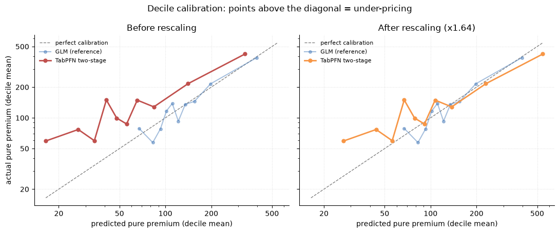
The two-stage TabPFN ranks well but under-prices the portfolio: summed over the test set it charges only ~60% of the actual claim cost. A log-link GLM never has this problem, fitting an intercept automatically balances its predicted total against the observed total on the training data. We can give TabPFN the same single degree of freedom: one constant factor = actual claim cost ÷ predicted cost, estimated on a calibration slice held out of training (never the test set). Because it is a constant, c · (p × s) orders policies exactly like p × s — so it fixes the level without moving the ranking one bit. One TabPFN-specific catch: TabPFN predicts by conditioning on its training rows in-context, so it effectively memorizes them — a policy it saw at fit time gets an unrealistically good prediction. Estimating the factor on such rows would under-correct, so we re-fit both stages on a subset (df_fit) and score the held-out slice (df_cal) they never saw.

# Calibration slice held out of TRAIN (never test); models re-fit WITHOUT it so the
# scored rows were not memorized in-context.
df_fit, df_cal = train_test_split(df_train, test_size=0.1, random_state=RANDOM_STATE)
X_fit = df_fit[tab_features]
X_cal_unit = df_cal[tab_features].copy()
X_cal_unit["Exposure"] = 1.0

clf_cal = TabPFNClassifier(n_estimators=N_ESTIMATORS, ignore_pretraining_limits=True)
clf_cal.fit(X_fit, (df_fit["ClaimAmount"] > 0).astype(int))
p_claim_cal = clf_cal.predict_proba(X_cal_unit)[:, list(clf_cal.classes_).index(1)]

pos_fit = (df_fit["ClaimAmount"] > 0).values
reg_cal = TabPFNRegressor(
    n_estimators=N_ESTIMATORS, ignore_pretraining_limits=True,
    inference_config={"REGRESSION_Y_PREPROCESS_TRANSFORMS": ("1_plus_log",)},
)
reg_cal.fit(X_fit[pos_fit], df_fit.loc[pos_fit, "ClaimAmount"])
severity_cal = reg_cal.predict(X_cal_unit)   # mean; plain predict avoids the full-output row cap

# One constant: actual claim cost / predicted cost on the held-out slice (exposure-weighted).
pp_cal = p_claim_cal * severity_cal
c = df_cal["ClaimAmount"].sum() / (pp_cal * df_cal["Exposure"]).sum()

pp_tabpfn_recal = c * pp_tabpfn                    # constant scaling: Gini unchanged

bal_before = (pp_tabpfn * weight).sum() / (pp_true * weight).sum()
bal_after = (pp_tabpfn_recal * weight).sum() / (pp_true * weight).sum()
print(f"rescale factor c = {c:.3f}")
print(f"portfolio balance (predicted / actual): {bal_before:.3f} -> {bal_after:.3f}")
scores(pp_tabpfn_recal)

rescale factor c = 1.637
portfolio balance (predicted / actual): 0.584 -> 0.956
{'Gini (exposure)  up': 0.32104571636786383,
 'D2 (Tweedie 1.9)  up': 0.00880833559375449,
 'Tweedie dev 1.9  down': 34.04750333782467,
 'Tweedie dev 1.5  down': 77.20614578550321}

The rescale is easiest to see decile by decile: bin the test policies by predicted premium and plot the predicted premium (x) against the actual claim cost (y) in each bin. Before, the two-stage points sit consistently above the diagonal — actual cost exceeds what the model charged, i.e. under-pricing; after the single constant factor they land on it. The GLM is drawn faintly in both panels for reference, and the ranking is identical between them — only the level moves.

from matplotlib.ticker import ScalarFormatter, NullFormatter, LogLocator


def decile_calibration(pred, n_bins=10):
    order = np.argsort(pred)
    exp = weight[order]
    edges = np.searchsorted(np.cumsum(exp) / exp.sum(), np.linspace(0, 1, n_bins + 1)[1:-1])
    pm, tm = [], []
    for g in np.split(order, edges):
        pm.append(np.average(pred[g], weights=weight[g]))
        tm.append(np.average(pp_true[g], weights=weight[g]))
    return np.clip(pm, 1e-1, None), np.clip(tm, 1e-1, None)

panels = [("Before rescaling", pp_tabpfn, "#c0504d"),
          (f"After rescaling (x{c:.2f})", pp_tabpfn_recal, "#f79646")]
gpm, gtm = decile_calibration(pp_glm_product)            # GLM reference, drawn in both panels
curves = {t: decile_calibration(pred) for t, pred, _ in panels}
allv = np.concatenate([gpm, gtm, *[v for pr in curves.values() for v in pr]])
lo, hi = allv.min(), allv.max()

fig, axes = plt.subplots(1, 2, figsize=(11, 4.6), sharex=True, sharey=True)
for ax, (title, _, color) in zip(axes, panels):
    pm, tm = curves[title]
    ax.plot([lo, hi], [lo, hi], "--", color="grey", lw=1, label="perfect calibration")
    ax.plot(gpm, gtm, "o-", color="#4f81bd", lw=1.5, ms=4, alpha=0.5, label="GLM (reference)")
    ax.plot(pm, tm, "o-", color=color, lw=2, ms=5, label="TabPFN two-stage")
    ax.set(xscale="log", yscale="log", title=title,
           xlabel="predicted pure premium (decile mean)")
    # Adaptive 1-2-5 decade ticks with plain-number labels; suppress crowded minor labels.
    for axis in (ax.xaxis, ax.yaxis):
        axis.set_major_locator(LogLocator(base=10, subs=(1, 2, 5)))
        axis.set_major_formatter(ScalarFormatter())
        axis.set_minor_formatter(NullFormatter())
    ax.grid(ls=":", alpha=0.4)
    ax.spines["top"].set_visible(False)
    ax.spines["right"].set_visible(False)
    ax.legend(frameon=False, fontsize=8, loc="upper left")
axes[0].set_ylabel("actual pure premium (decile mean)")
fig.suptitle("Decile calibration: points above the diagonal = under-pricing")
plt.tight_layout()
plt.show()

Optional: matching the GLM on calibration

Results

All five models side by side, then the Lorenz curves for the ranking view (calibration was covered in the section above).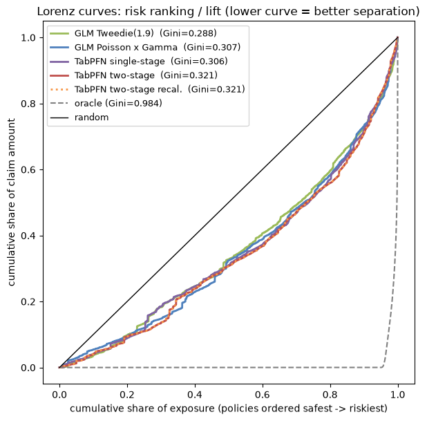

table = pd.DataFrame({
    "GLM Tweedie(1.9)": scores(pp_glm_tweedie),
    "GLM Poisson x Gamma": scores(pp_glm_product),
    "TabPFN single-stage": scores(pp_tabpfn_single),
    "TabPFN two-stage": scores(pp_tabpfn),
    "TabPFN two-stage recal.": scores(pp_tabpfn_recal),
})
table.round(4)

                       GLM Tweedie(1.9)  GLM Poisson x Gamma  \
Gini (exposure)  up              0.2883               0.3067
D2 (Tweedie 1.9)  up             0.0137               0.0146
Tweedie dev 1.9  down           33.8783              33.8483
Tweedie dev 1.5  down           76.4087              76.1599

                       TabPFN single-stage  TabPFN two-stage  \
Gini (exposure)  up                 0.3063            0.3210
D2 (Tweedie 1.9)  up               -0.1561           -0.0226
Tweedie dev 1.9  down              39.7118           35.1277
Tweedie dev 1.5  down              98.8292           82.2073

                       TabPFN two-stage recal.
Gini (exposure)  up                     0.3210
D2 (Tweedie 1.9)  up                    0.0088
Tweedie dev 1.9  down                  34.0475
Tweedie dev 1.5  down                  77.2061

Lorenz curves. Policies are sorted safest → riskiest by predicted premium; we plot the cumulative share of actual claim cost against the cumulative share of exposure. A lower, more bowed curve means better risk separation. Two reference lines frame it: random (the diagonal) and the oracle (sorted by realized losses — Gini ~0.98, not 1.0, because claim-bearing policies still occupy a few percent of the exposure axis). No expected-risk model can reach the oracle: realized claims are mostly luck, and a model can only rank who is riskier on average. The recalibrated two-stage curve overlays the uncalibrated one exactly — constant rescaling never reorders a single policy.

fig, ax = plt.subplots(figsize=(6.2, 6.2))
curves = [
    ("GLM Tweedie(1.9)", pp_glm_tweedie, "#9bbb59", "-"),
    ("GLM Poisson x Gamma", pp_glm_product, "#4f81bd", "-"),
    ("TabPFN single-stage", pp_tabpfn_single, "#8064a2", "-"),
    ("TabPFN two-stage", pp_tabpfn, "#c0504d", "-"),
    # Constant rescaling preserves the ordering, so this overlays two-stage exactly.
    ("TabPFN two-stage recal.", pp_tabpfn_recal, "#f79646", ":"),
]
for label, pred, color, ls in curves:
    order = np.argsort(pred)
    exp = weight[order]
    claim = pp_true[order] * exp
    cx = np.insert(np.cumsum(exp) / exp.sum(), 0, 0)
    cy = np.insert(np.cumsum(claim) / claim.sum(), 0, 0)
    ax.plot(cx, cy, color=color, lw=2, ls=ls,
            label=f"{label}  (Gini={gini_exposure(pp_true, pred, weight):.3f})")

order = np.argsort(pp_true)                          # oracle
exp = weight[order]; claim = pp_true[order] * exp
ax.plot(np.insert(np.cumsum(exp) / exp.sum(), 0, 0),
        np.insert(np.cumsum(claim) / claim.sum(), 0, 0),
        "--", color="grey", label=f"oracle (Gini={gini_exposure(pp_true, pp_true, weight):.3f})")
ax.plot([0, 1], [0, 1], color="black", lw=1, label="random")

ax.set_xlabel("cumulative share of exposure (policies ordered safest -> riskiest)")
ax.set_ylabel("cumulative share of claim amount")
ax.set_title("Lorenz curves: risk ranking / lift (lower curve = better separation)")
ax.legend(loc="upper left", fontsize=9)
plt.tight_layout()
plt.show()

Takeaways

Better ranking, zero feature engineering. From the raw 9-column dataframe — strings and all, one .fit() / .predict() — TabPFN reaches Gini ~0.32 vs ~0.31 for the best GLM. The GLM needed a hand-built 75-column design matrix (binning, one-hot, log-scaling) and several modeling choices to get there.
Uncertainty comes built in. TabPFN returns a full predictive distribution per policy, so you read off the expected claim and its tail (the P90 “bad case”) directly — exactly what risk loading and capital planning need. The GLM gives a mean and stops.
Calibration is a one-liner away. Out of the box TabPFN under-prices the portfolio (it has no exposure offset, a genuine convenience the GLMs keep). A single portfolio-level factor — the same balancing a log-link GLM performs implicitly — restores the level (balance ~0.6 → ~0.96) and brings the Tweedie deviance in line with the GLMs, while provably leaving the ranking untouched.
The two-stage split helps TabPFN too. Occurrence × severity is better calibrated than a single regressor on the raw zero-inflated amount — the classic actuarial decomposition still pays off.
Match the metric to the question. Judge ranking with the exposure-weighted Gini (the headline for pricing) and calibration with Tweedie deviance / D² and the decile chart. MAE and RMSE are actively misleading on a 96%-zero, heavy-tailed target.

​The data

​Metrics

​GLM baselines

​Single-stage GLM: direct Tweedie on pure premium

​Two-stage GLM: frequency × severity

​TabPFN

​Single-stage TabPFN: regress the claim amount directly

​Two-stage TabPFN: occurrence × severity

​Per-policy uncertainty: the whole distribution, not just a number

​Optional: matching the GLM on calibration

​Results

​Takeaways