
Setup
Load a panel of related series
We use Favorita Store Sales, accessed through a public mirror. The prepared teaching panel is included in this repository; its source snapshot and checksum are fixed for reproducibility. Sales are quantities, not revenue; some families include quantities measured by weight. The subset is fixed before evaluating forecasts: stores 1–12 and BEVERAGES, BREAD/BAKERY, CLEANING, and GROCERY I. These 48 store–family series form four groups of 12. We retain roughly two years of training history plus earlier observations for lag construction. This is a teaching subset, not a benchmark of the full competition. Holiday features respect city/state/national scope and transferred dates. Future promotion counts are treated as plans known at the origin, matching the competition’s provision of future promotions; the historical file does not preserve plan revisions. Realized future oil prices and transaction counts are excluded.Two series and a forecast origin
We pick two series as an example. At an origin , sales through are observed. Dates, calendar features, and planned promotions for through are available. Sales in that window are labels used only for scoring.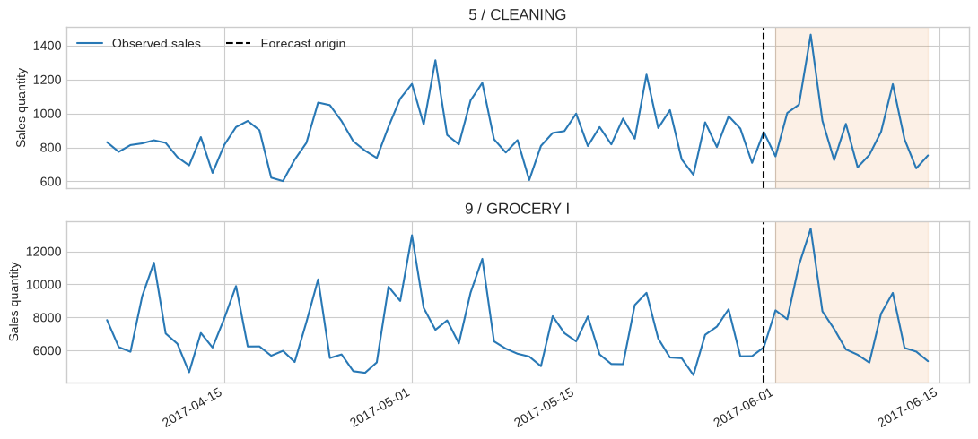
Start with ordinary date features
A date becomes year, month, day of month, weekday, and a time index. Add the same known covariates and static identifiers that we will keep in later models.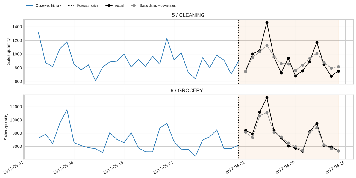
Add Fourier terms to describe repeating seasons
For each period , add and . We use two harmonics for the weekly and annual cycles: eight extra columns. These depend only on the target date and remain available at any forecast horizon. Everything else stays the same, including promotions, training dates, model settings, and held-out targets.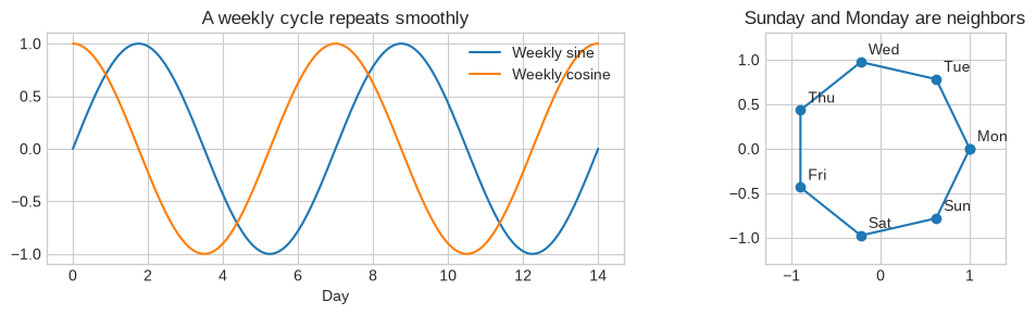
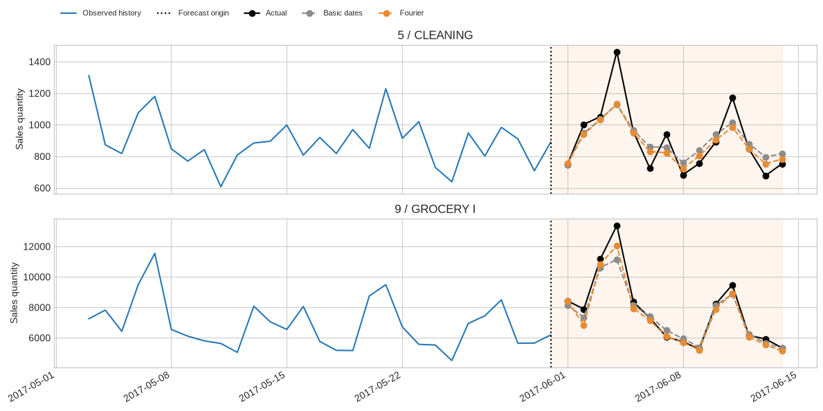 Adding Fourier terms reduces MAE for both illustrated series. Some peaks remain underestimated.
Add observed history to predict two days ahead
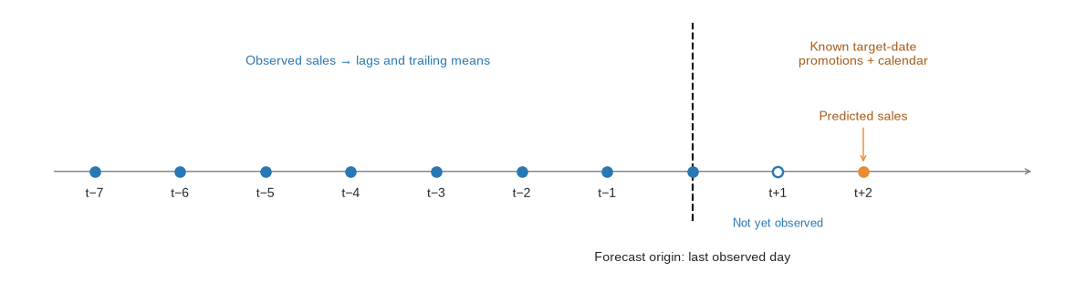
A supervised row now has two dates: origin and target date. At origin ,last_sales is ; sales_7d_ago is ; the trailing means end at . Promotions, Fourier terms, and calendar features belong to the target date .
The training label is . A training row is eligible only when its label date is at or before the current forecast cutoff.
The helper also removes rows with incomplete sales history from both training data and forecast queries. All 48 series have the required history at the evaluation origins used here, but a series with incomplete recent history would be omitted by this helper. When adapting the example, check that every requested series and horizon has a prediction, and choose an explicit missing-history policy before using the forecasts.
Forecast all 14 horizons directly
The two-day-ahead model above is already a direct forecast: it maps observed history at origin and known target-date covariates to sales at . We now repeat that construction for every horizon . The distinction is between origin-relative and target-relative lags. Sales two days before the origin, , are known for every forecast horizon. A two-day lag relative to the target would instead be ; for , that requires , which is not yet observed. Our features are origin-relative, so the same observed sales history is available for all 14 horizons. This implementation fits a separate model for each horizon. Historical rows pair history at an origin with the label days later, and only labels observed by the current cutoff enter training. Query rows share the history through , while their target-date calendar and promotion features change with . No predicted sales are fed into another horizon’s history. Separate fits are a modeling choice, not a requirement imposed by lag features; the existing fit is reused. For our two illustrated series this requires 2 × 14 = 28 fits, compared with 2 fits for either calendar-only method.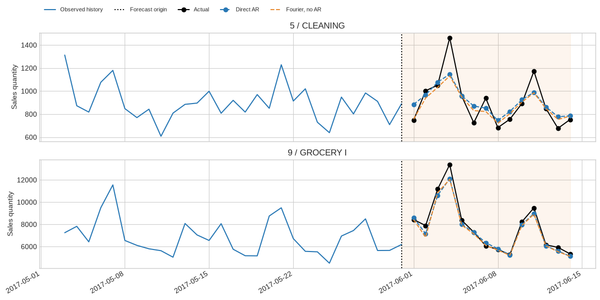
Share the context across related series
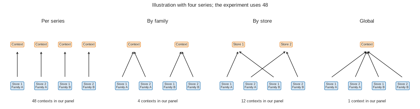
Pooling related series lets TabPFN learn from their shared patterns. This changes which rows TabPFN sees, not the forecast target. Each query still predicts one store–family series. Identifiers remain features so a shared model can distinguish stores and families.- Per series: each context contains one store–family history.
- By family: each context contains 12 stores selling the same family.
- By store: each context contains the four families sold at one store.
- Global: one context contains all 48 series.
How many fits?
Counts below are per forecast origin. “Fit” means one scikit-learnfit call that establishes a TabPFN context; it does not mean training the foundation model’s weights. Each call may internally use an ensemble.
Here series, families, stores, and . Across three test origins, each no-AR method needs 195 fits across all pooling strategies; direct AR needs 2,730 fits. The main comparison therefore needs 3,120 fits. The results are reused from direct AR, not fitted again. The two-series walkthrough adds 32 fits, plus one excluded warm-up.
Evaluate three future windows
Use the origins June 30, July 14, and July 28, 2017. Each forecast covers the next 14 days without observing any sales inside that window. At the next origin, previously observed sales may enter history. Each backtest uses a fixed 730-day training window and keeps the forecast origin unchanged throughout the forecast window. The primary score is mean per-series seasonal MASE: absolute forecast errors are divided by each series’ training-only mean absolute seven-day difference, then averaged equally across series and origins. Zero-denominator series are reported and excluded from scaled scores for every method. We also report average within-series rank and the fraction of series won. Weekly seasonal-naive repeats the last observed week as a reference.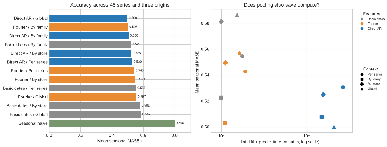
Compare pooling within each feature method
Average rank and win share below compare only the four pooling strategies within each method. First average errors over origins and horizons for each series, then rank. Tied wins share their weight, so the four win shares sum to 100%.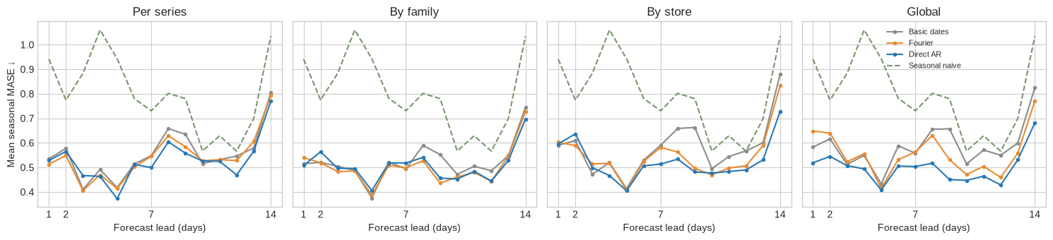 Global direct AR has the lowest test MASE and takes less model time than per-series direct AR. Fourier features improve mean test MASE across the pooling strategies.
Family pooling is particularly useful for the Fourier model: its accuracy is close to global direct AR, with much less fit-and-predict time.
Store pooling also improves direct AR accuracy and reduces model time relative to per-series fits. Global pooling improves direct AR but hurts the non-autoregressive methods, so validate the feature representation and pooling level together.
Global direct AR has the lowest test MASE and takes less model time than per-series direct AR. Fourier features improve mean test MASE across the pooling strategies.
Family pooling is particularly useful for the Fourier model: its accuracy is close to global direct AR, with much less fit-and-predict time.
Store pooling also improves direct AR accuracy and reduces model time relative to per-series fits. Global pooling improves direct AR but hurts the non-autoregressive methods, so validate the feature representation and pooling level together.