ByEliott Kalfon

Time-Series Forecasting with TabPFN

Turning the tabular foundation model into a zero-shot forecaster. TabPFN can forecast time series without any task-specific training. The tabpfn-time-series package wraps the model in a pipeline that takes historical context and returns a probabilistic forecast. This notebook covers both a univariate forecast on the M4 hourly dataset and a multivariate forecast, where known future covariates sharpen the prediction. Reference: https://github.com/PriorLabs/tabpfn-time-series/blob/main/examples/quickstart.ipynb

Setup

Installing the time-series package and authenticating. tabpfn-time-series brings the pipeline and plotting helpers. As elsewhere, the API token is read from Colab secrets.

!pip install scikit-learn tabpfn-time-series

import os

import pandas as pd

from google.colab import userdata
from tabpfn_time_series import TabPFNTSPipeline, TabPFNMode
from tabpfn_time_series.plot import plot_forecast

Authenticating with a Token

Setting TABPFN_TOKEN so the pipeline can reach the TabPFN API. As elsewhere, the API token is read from Colab secrets. Accept the license and copy your key from priorlabs.ai if you have not already.

from tabpfn_client import set_access_token
set_access_token(userdata.get('TABPFN_TOKEN'))

Loading the Data

The M4 hourly dataset: many hourly series with a known future to score against. The M4 dataset is a standard forecasting benchmark from the M4 competition; its hourly subset is a collection of many independent hourly time series (things like electricity demand or web traffic). Each individual series is one item, identified by an item_id, and we forecast each one separately. We load the standard M4 hourly train and test splits: the train frame is the historical context, and the test frame holds the actual future values we will compare the forecast against.

# Load M4 Hourly dataset
m4_hourly_train_url = (
    "https://autogluon.s3.amazonaws.com/datasets/timeseries/m4_hourly/train.csv"
)
m4_hourly_test_url = (
    "https://autogluon.s3.amazonaws.com/datasets/timeseries/m4_hourly/test.csv"
)
m4_train_df = pd.read_csv(m4_hourly_train_url, parse_dates=["timestamp"])
m4_test_df = pd.read_csv(m4_hourly_test_url, parse_dates=["timestamp"])

m4_train_df.head()

  item_id           timestamp  target
    H1 1750-01-01 00:00:00   605.0
    H1 1750-01-01 01:00:00   586.0
    H1 1750-01-01 02:00:00   586.0
    H1 1750-01-01 03:00:00   559.0
    H1 1750-01-01 04:00:00   511.0

Select a few series

Restricting to two items to keep the demo fast and legible.

selected_items = m4_train_df["item_id"].unique()[:2]
context_df = m4_train_df[m4_train_df["item_id"].isin(selected_items)].copy()
test_df = m4_test_df[m4_test_df["item_id"].isin(selected_items)].copy()

print("context_df.shape", context_df.shape)
context_df.tail()

context_df.shape (1400, 3)
     item_id           timestamp  target
    H2 1750-01-29 23:00:00  3705.0
    H2 1750-01-30 00:00:00  3652.0
    H2 1750-01-30 01:00:00  3460.0
    H2 1750-01-30 02:00:00  3248.0
    H2 1750-01-30 03:00:00  3105.0

Build the pipeline

One pipeline object drives both the univariate and multivariate forecasts. By default TabPFNTSPipeline runs TabPFN through the hosted API (tabpfn-client) rather than a local model. That is why the progress logs further down come from the client, and why the TABPFN_TOKEN set above is what authenticates those calls.

pipeline = TabPFNTSPipeline(tabpfn_mode=TabPFNMode.CLIENT)

Univariate Forecast

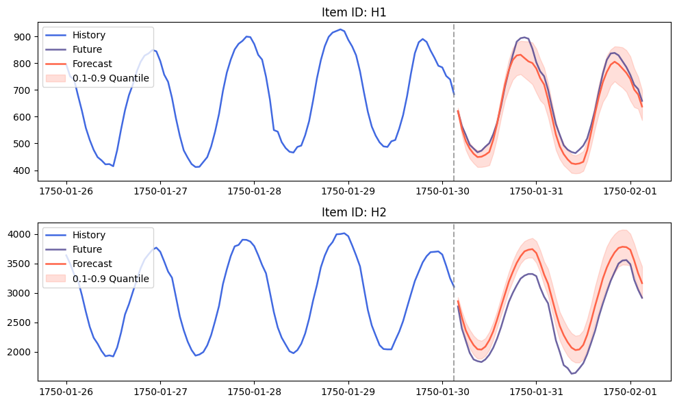
Forecasting from history alone, with no extra inputs. We ask the pipeline for a 48-step horizon. With only context_df, each series is forecast purely from its own past. The result is probabilistic, with quantiles around the median.

prediction_length = 48

pred_df = pipeline.predict_df(
    context_df=context_df,
    prediction_length=prediction_length,
)

print("pred_df.shape", pred_df.shape)
pred_df.head()

pred_df.shape (96, 10)
                                 target         0.1         0.2         0.3  \
item_id timestamp
H1      1750-01-30 04:00:00  621.089050  608.086243  613.247009  616.246643
        1750-01-30 05:00:00  554.764526  532.325439  541.405579  547.201721
        1750-01-30 06:00:00  508.915863  476.036377  489.271973  498.152802
        1750-01-30 07:00:00  480.749176  444.337830  457.773895  467.694153
        1750-01-30 08:00:00  461.458160  426.360077  439.234741  449.052673

                                    0.4         0.5         0.6         0.7  \
item_id timestamp
H1      1750-01-30 04:00:00  618.930969  621.089050  623.311768  625.763611
        1750-01-30 05:00:00  551.278687  554.764526  558.151489  561.748901
        1750-01-30 06:00:00  504.377045  508.915863  512.794189  516.848633
        1750-01-30 07:00:00  475.012909  480.749176  485.107788  489.648529
        1750-01-30 08:00:00  456.048645  461.458160  466.238739  471.229492

                                    0.8         0.9
item_id timestamp
H1      1750-01-30 04:00:00  628.593567  632.677734
        1750-01-30 05:00:00  566.105591  572.157654
        1750-01-30 06:00:00  521.319580  528.396179
        1750-01-30 07:00:00  494.574799  501.992279
        1750-01-30 08:00:00  476.649323  483.684204

Plotting the forecast

The forecast against the held-out actuals. plot_forecast overlays the predicted median and quantile band on the historical context and the true future values.

test_df = test_df.groupby("item_id").tail(prediction_length)
plot_forecast(context_df, pred_df, test_df=test_df, item_ids=selected_items)

Multivariate Forecast

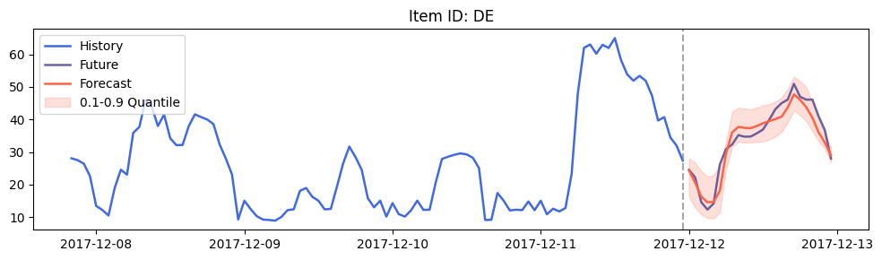
Adding known future covariates to sharpen the prediction. Often we know something about the future: a load forecast, a weather forecast. The pipeline can condition on these covariates. Here we use an electricity-price dataset that ships with related forecasts, and compare predictions with and without them.

Load the data

The electricity-price dataset, with covariate columns alongside the target.

# Load Electricity Price dataset
train_url = "https://autogluon.s3.amazonaws.com/datasets/timeseries/electricity_price/train.parquet"
test_url = "https://autogluon.s3.amazonaws.com/datasets/timeseries/electricity_price/test.parquet"

elec_train_df = pd.read_parquet(train_url)
elec_test_df = pd.read_parquet(test_url)

print(f"Train shape: {elec_train_df.shape}")
print(f"Test shape: {elec_test_df.shape}")
print(f"\nColumns: {elec_train_df.columns.tolist()}")
elec_train_df.head()

Train shape: (51936, 5)
Test shape: (24, 5)

Columns: ['id', 'timestamp', 'target', 'Ampirion Load Forecast', 'PV+Wind Forecast']
   id           timestamp     target  Ampirion Load Forecast  PV+Wind Forecast
0  DE 2012-01-09 00:00:00  34.970001                16382.00       3569.527588
1  DE 2012-01-09 01:00:00  33.430000                15410.50       3315.274902
2  DE 2012-01-09 02:00:00  32.740002                15595.00       3107.307617
3  DE 2012-01-09 03:00:00  32.459999                16521.00       2944.620117
4  DE 2012-01-09 04:00:00  32.500000                17700.75       2897.149902

Prepare the data

Renaming to the expected schema and isolating a single region. The pipeline expects timestamp, target, an optional item_id, and any covariate columns. We rename accordingly, pick one region, and split the covariates into a future_df that excludes the target.

# Rename columns to match expected format
# The pipeline expects: timestamp, target, item_id (optional), and any covariate columns
elec_train_df = elec_train_df.rename(columns={"id": "item_id"})
elec_test_df = elec_test_df.rename(columns={"id": "item_id"})
covariate_cols = ["Ampirion Load Forecast", "PV+Wind Forecast"]

# Select a single region for demonstration.
# You can pass multiple item_ids here as long as future_df contains each item's horizon covariates.
selected_region = elec_train_df["item_id"].unique()[0]
context_df = elec_train_df[elec_train_df["item_id"] == selected_region].copy()
test_df = elec_test_df[elec_test_df["item_id"] == selected_region].copy()

print(f"Region: {selected_region}")
print(f"Context length: {len(context_df)}")
print(f"Test length: {len(test_df)}")

Region: DE
Context length: 51936
Test length: 24

future_df = test_df.drop(columns=["target"])

print("Future covariates:")
future_df.head()

Future covariates:
  item_id           timestamp  Ampirion Load Forecast  PV+Wind Forecast
    DE 2017-12-12 00:00:00                20483.00      22284.005859
    DE 2017-12-12 01:00:00                19849.75      22878.673828
    DE 2017-12-12 02:00:00                19638.25      23632.283203
    DE 2017-12-12 03:00:00                19895.25      24635.945312
    DE 2017-12-12 04:00:00                20338.00      25584.935547

Predict with and without covariates

Two forecasts from the same history, differing only in the covariates. Running the pipeline twice, once including the covariate columns and once dropping them, isolates exactly how much the extra information helps.

pred_w_covariates_df = pipeline.predict_df(
    context_df=context_df,
    future_df=future_df,
)
pred_without_covariates_df = pipeline.predict_df(
    context_df=context_df.drop(columns=covariate_cols),
    future_df=future_df.drop(columns=covariate_cols),
)

Comparing the Forecasts

Side by side: does knowing the future help?

Without covariates

History only.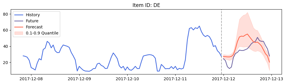

plot_forecast(
    context_df, pred_without_covariates_df, test_df=test_df, item_ids=[selected_region]
)

With covariates

The same horizon, now conditioned on the known future inputs.

plot_forecast(
    context_df, pred_w_covariates_df, test_df=test_df, item_ids=[selected_region]
)

​Time-Series Forecasting with TabPFN

​Setup

​Authenticating with a Token

​Loading the Data

​Select a few series

​Build the pipeline

​Univariate Forecast

​Plotting the forecast

​Multivariate Forecast

​Load the data

​Prepare the data

​Predict with and without covariates

​Comparing the Forecasts

​Without covariates

​With covariates