
We first build intuition on a small toy example. Then we compare the three methods on two real datasets from ScoringBench, a benchmark for probabilistic regression.
Setup
Install the TabPFN client and the usual scientific Python stack. TabPFN runs on Prior Labs’ servers through the API.A toy example: plants in the sun
We start with made-up data, so that we know the true answer. Each plant gets some hours of sunlight per day. We want to predict two targets: its height and its width (in cm).- More sun makes a plant both taller and wider on average.
- Even for the same sunlight, plants differ. A plant that is taller than usual is also, most of the time, wider than usual. We set the correlation of these “surprises” to 0.85.
One target: TabPFN predicts a whole distribution
Let us first predict only the height. TabPFN does not just return one number. Withoutput_type="full" it returns a probability for each of 5,000 small intervals (“bars”) of possible heights. Together they form the predictive distribution: which heights are likely for this plant, and how sure the model is.
Below, we ask about a new plant with 6 hours of sunlight. The true height for such a plant is 15 cm on average, with a spread (standard deviation) of 2 cm.
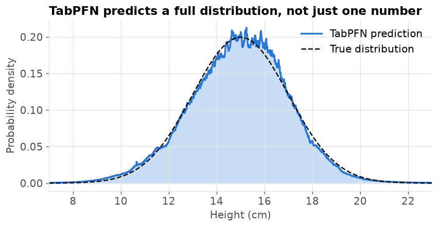 In this recipe we read these distributions through their quantiles. The 30% quantile is the height that the plant is below with 30% probability. With quantiles at many levels (0.5%, 1%, …, 99.5%) we can do two useful things:
- Draw random samples. Pick a random percentile, for example 72%, and read off the value at that quantile. Repeat this many times and you get a cloud of plausible outcomes.
- Find where a real value falls. Given an observed height, find its percentile in the predicted distribution. We use this for the copula below.
percentiles is an array of numbers between 0 and 1.
Three ways to predict two targets together
A joint prediction answers “which (height, width) pairs are likely?”. We will represent it by drawing, say, 200 plausible pairs for each plant. A good joint prediction has two properties: each target on its own is right (the marginals), and the targets move together in the right way (the dependence).1. Independent
Fit one TabPFN model for height and one for width, each from sunlight only. To draw a pair, draw a height from the height model and, separately, a width from the width model. A worked example for a plant with 6 hours of sun. Say the height model predicts “about 15 cm, give or take 2” and the width model “about 5.8 cm, give or take 1”. Four independent draws could look like this:
Each column on its own is fine. But draws 1, 2 and 4 combine a tall plant with a narrow one, or the other way round. In our data such plants are rare, because the surprises are correlated. The independent method throws this information away.
2. Chained
Use the rule from probability: P(height, width) = P(height) × P(width given height).- Model 1 predicts height from sunlight (the same model as before).
- Model 2 predicts width from sunlight and the true height. During training we know both targets, so we can give the true height to model 2 as an extra input column.
Now a tall plant gets a wide width, and the spread of model 2 is smaller, because knowing the height tells it a lot. The price: model 2 must make a prediction for every draw (200 draws × number of plants), and the result can depend on which target we put first.
3. Copula
Keep the two independent models, and learn one extra number (or a small matrix for more targets) that describes how their errors move together. A copula is this “glue” between distributions. We use the simplest one, the Gaussian copula, in four steps:- Percentiles of the truth. For each training plant, find where its true height falls in its predicted height distribution, for example at the 84th percentile. Do the same for width.
- Normal scores. Turn each percentile into a z-score of a standard normal distribution: 50% → 0, 84% → 1.0, 16% → -1.0.
- Correlation. Compute the correlation of the height z-scores with the width z-scores over all training plants. If tall-for-its-sunlight plants are also wide-for-their-sunlight, this correlation is high.
- Sampling. Draw pairs of correlated z-scores with that correlation, turn them back into percentiles, and read each target’s prediction at its percentile.
The two z columns go up and down together, so their correlation is high (about 0.97 here). When we sample, a plant drawn at the 90th height percentile will usually also be drawn at a high width percentile.
One detail matters for step 1. TabPFN learns from the training rows it is given (its “context”). If a plant is in the context, the model has already seen its true height, so the percentile is too close to 50% and the correlation would be wrong. We therefore compute each training plant’s percentile with a model that did not see it: we split the training data into 5 parts and, for each part, use a model fitted on the other 4 parts. This is called cross-fitting.
The three methods on the toy plants
We fit all three on the 300 toy plants and draw 400 (height, width) pairs for a new plant with 6 hours of sunlight. Because the data is made up, we can also draw from the true joint distribution and compare.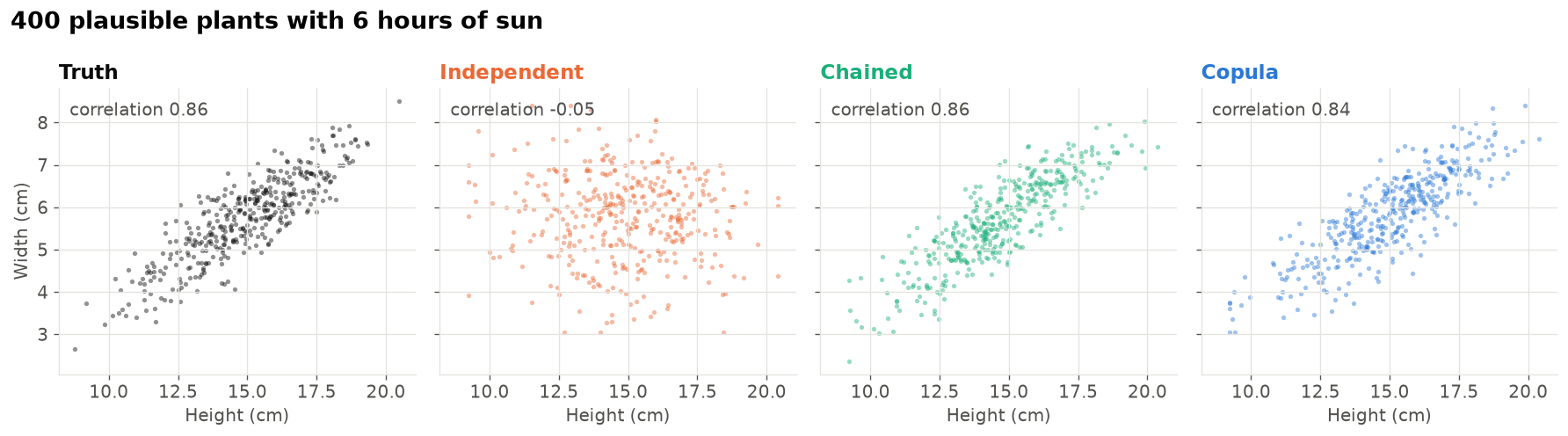 All four clouds have about the same horizontal and vertical spread: each target on its own is predicted well by every method. The difference is the shape. The true cloud is a tilted ellipse. The independent cloud is round, because it ignores the link between height and width. The chained and copula clouds recover the tilt.
How to score a joint prediction
We need one number that says how good a cloud of draws is, given the real outcome. We use the energy score. For one row with true outcome y and draws x₁, …, xₘ: energy score = (average distance from a draw to the truth) − ½ × (average distance between two draws)- The first part rewards clouds that are close to the truth.
- The second part rewards clouds that are spread out. Without it, the best strategy would be to put every draw on one confident point. The two parts together reward a cloud that is exactly as wide as it needs to be.
- Lower is better. Distances are Euclidean, so all targets count together.
Average distance to the truth: (1 + 1 + 1.41) / 3 = 1.14. Distances between pairs of draws: x₁–x₂ = 1.41, x₁–x₃ = 1, x₂–x₃ = 1, average 1.14. Energy score = 1.14 − ½ × 1.14 = 0.57.
With a single target, the energy score is the well-known CRPS (continuous ranked probability score). We report the CRPS of each target too. It only looks at one target at a time, so it tells us whether a method gets the marginals right, independently of the dependence.
Targets can have very different units, so before scoring we convert each target to standard units: subtract the training mean and divide by the training standard deviation.
Real data from ScoringBench
We use two small multi-target datasets from the ScoringBench multivariate list, loaded from OpenML. Both have strongly linked targets. Weather in Ankara (OpenML 42368). 321 days of weather measurements. The targets are the day’s minimum temperature, maximum temperature and dew point (the temperature at which dew forms, a measure of humidity), all converted to °C. The inputs are the other measurements of the same day: precipitation, air pressure, visibility and wind speed. Like ScoringBench, we drop the mean temperature (it would give the answer away) and the maximum wind speed. The minimum temperature is never above the maximum temperature, so this dataset can also show us how often each method produces impossible days. Skin lesions (OpenML 46630, from the PAD-UFES-20 dataset). Patient information and symptoms for skin lesions photographed with smartphones. The two targets are the lesion’s two diameters in mm. The inputs include age, skin type, body region, the diagnosis and symptoms such as itching or bleeding. We keep the 1,494 images with both diameters (one row per image) and drop the identifier columns. Why we split by patient. The rows are not independent. The 1,494 images come from 1,134 lesions and 794 patients. 314 lesions were photographed more than once, and these repeat rows have exactly the same diameters. Many inputs, such as age, skin type and family history, are also the same for every row of a patient. With a random row split, a copy of a test lesion would often be in the training data, and the model could simply look up its diameters: the score would look much better than it would be for a new patient. So we useGroupKFold with patient_id as the group: all rows of one patient are either in the training data or in the test data, never in both. The inner split that fits the copula correlation is grouped in the same way. Only the split uses the patient: the model still trains and predicts one row (one image) at a time, and the scores are averaged over rows.
We evaluate each dataset with 5-fold cross-validation: every row is a test row exactly once, predicted by models that never saw it.
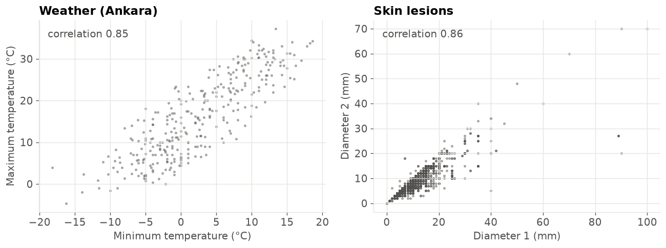 These correlations mix two things: the part the inputs explain (a sunny day is warm both at night and in the afternoon) and the part they do not. Only the second part, the link between the surprises, can help a joint model beat the independent one.
Run the comparison
For each fold we fit the models on the training rows, draw 200 joint samples for every test row with each method, and score them. For the chained method we keep the target order shown above. The same random number generator is used throughout so that the run is reproducible.Results
Energy score
The table shows the energy score averaged over the five folds (lower is better). The chart shows the change relative to the independent method, in percent: below zero means better than independent. Each dot is one fold.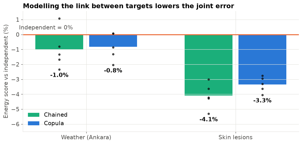 Both joint methods beat the independent method on both datasets. On the skin lesions the gain is clear and holds in every fold. On the weather data it is small: most folds improve, but one fold of each method is level with independent or slightly worse. The chained method is a little ahead of the copula on both datasets.
Each target on its own
The CRPS of each target checks the marginals. The independent and copula methods use exactly the same marginal distributions, so they differ only by random sampling noise. The chained method has different marginals for every target after the first one, because those targets are predicted from drawn values of the earlier targets.Impossible weather days
On a real day, the minimum temperature is never above the maximum. How often does each method still draw such a day?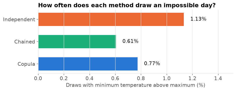 Impossible days are rare for every method, because the predicted minimum is usually well below the predicted maximum. Still, the independent method draws them most often, roughly twice as often as the chained method. The copula sits in between. Neither joint method removes them completely: they learn that the two temperatures move together, not the hard rule that one is always below the other.
What the joint predictions look like
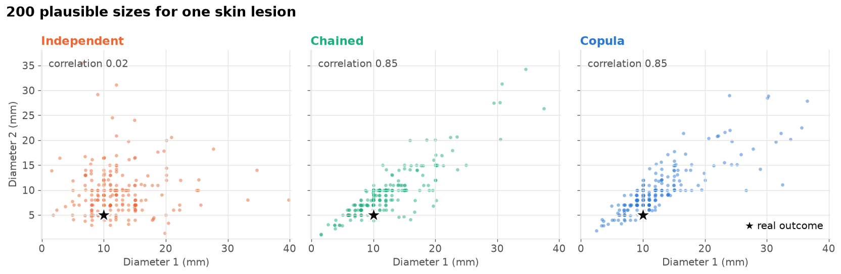
For one test row of each dataset we plot the 200 draws of each method together with the real outcome (black star). We pick a typical row: the one whose independent predictions have the median spread. For the weather we show minimum temperature against dew point, the pair with the strongest link (see the next section). Axes show the central 98% of the draws.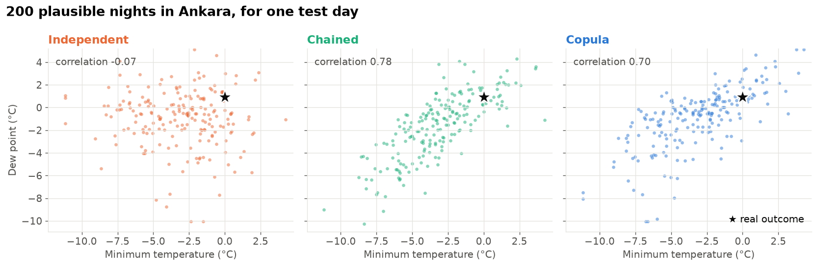
The glue the copula learns
The copula’s correlation describes how the surprises move together. We can check it on the test rows: for each test row, take the percentile of the true value in the independent prediction, for each target. If the targets’ surprises were unrelated, these points would fill the square evenly. Points along the diagonal mean “when one target is higher than predicted, the other one is too”.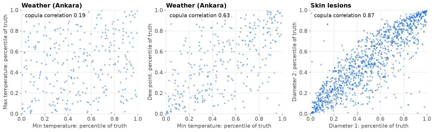 The three panels explain the size of the gains. For the skin lesions the points lie along the diagonal, and the copula learns a strong correlation: a lesion that is longer than predicted is almost always wider than predicted too. For the weather, the surprises of the minimum and maximum temperature are only weakly linked, so knowing one tells us little about the other. The minimum temperature and the dew point are more strongly linked. The weaker the glue, the less a joint model can gain over the independent one.
Which method should you use?
- Independent is the simplest and cheapest: one model per target. It is the right choice when you only use each target on its own, for example a separate prediction interval for each one. It gives the same per-target quality as the other two methods.
- Chained gave the best joint predictions here. It needs one model per target, but every model after the first must predict once per draw: with 200 draws, 200 times as many rows. Its result can also depend on the target order. Trying a few orders, or putting the easiest target first, is a good habit.
- Copula keeps the independent predictions and adds the link between targets with a few extra fits during training (the cross-fitting). Sampling is then almost free, and the method does not depend on any target order. The Gaussian copula describes the link with correlations only, so it cannot capture, for example, a link that only appears for extreme values. Vine copulas, which ScoringBench uses, are a more flexible option.